WIXLIB

Fatigue Life Estimates Using Goodman Diagramsby Robert StoneThe purpose of this paper is to review the proper methods by which spring manufacturers should estimatethe fatigue life of a helical compression springs during the design phase. The paper will begin with aworking definition of fatigue and a brief discussion of fatigue characteristics. A short history will bepresented as to how fatigue test data has been evaluated historically (e.g., S-N curves, Weibull distribution,modified Goodman diagrams, etc.) Spring-specific Modified Goodman diagrams, presented in the newSMI Encyclopedia of Spring Design, will be discussed. These Modified Goodman diagrams have beensufficiently characterized to facilitate direct calculation of predicted life. These calculations will bepresented along with a comparison to the results of traditional graphical methods.An Overview of FatigueFatigue, or metal fatigue, is the failure of a component as a result of cyclic stress. The failure occurs inthree phases: crack initiation, crack propagation, and catastrophic overload failure. The duration of each ofthese three phases depends on many factors including fundamental raw material characteristics, magnitudeand orientation of applied stresses, processing history, etc. Fatigue failures often result from applied stresslevels significantly below those necessary to cause static failure.Fatigue failures are typically characterized as either low-cycle ( 1,000 cycles) or high-cycle ( 1,000cycles). The threshold value dividing low- and high-cycle fatigue is somewhat arbitrary, but is generallybased on the raw material’s behavior at the microstructural level in response to the applied stresses. Lowcycle failures typically involve significant plastic deformation. An example would be reversed 90 bendingof a paperclip. Gross plastic deformation will take place on the first bend, but failure will not occur untilapproximately 20 cycles. Plastic deformation does play a role in high cycle fatigue; however, the plasticdeformation is very localized and not necessarily discernable by a macroscopic evaluation of thecomponent. In summary, while a valve spring designer may consider a failure at 10,000 cycles very shortlife, the failure can still be the result of high-cycle fatigue because the material response at themicrostructural level is the same as in a 10,000,000-cycle failure under lower applied stresses.Most metals with a body centered cubic crystal structure have a characteristic response to cyclic stresses.These materials have a threshold stress limit below which fatigue cracks will not initiate. This thresholdstress value is often referred to as the endurance limit. In steels, the life associated with this behavior isgenerally accepted to be 2x106 cycles. In other words, if a given stress state does not induce a fatiguefailure within the first 2x106 cycles, future failure of the component is considered unlikely. For springapplications, a more realistic threshold life value would be 2x107 cycles. Metals with a face center cubiccrystal structure (e.g. aluminum, austenitic stainless steels, copper, etc.) do not typically have an endurancelimit. For these materials, fatigue life continues to increase as stress levels decrease; however, a thresholdlimit is not typically reached below which infinite life can be expected.The S-N CurveThe discussion above touched on the relationship between applied stress and expected life. For thedesigner, it is critical that this relationship be characterized so that fatigue life can be predicted. One of theearly methods for characterizing this relationship is the S-N curve. ‘S’ stands for the cyclic stress rangewhile ‘N’ represents the number of cycles to failure.To develop the curve, a series of samples is tested to failure at various stress ranges. The resulting lives areplotted versus the corresponding stress range. The S-N curve is the locus of these data points. In morethorough testing, multiple samples are tested at each stress range. Common practice is to plot the S-Ncurve through the mean value at each stress range. An example is shown in Figure 1. Note that in thiscase, a fatigue stress below 49 kpsi will not induce failure.

Figure 1. An S-N diagram plotted from the results of completely reversed axial fatigue tests.Material: UNS G41300 steel normalized; Sut 116 kpsi; maximum Sut 125 kpsi. (Data from NACATechnical Note 3866, December 1966.)1One significant limitation of the S-N curve is that the resulting plot is highly dependent on the testconditions (e.g. the stress ratio Smin/Smax, sample geometry, sample surface condition, and material). Usingan S-N curve to predict real-world life when conditions do not match the test conditions under which thecurve was developed is dubious at best. This severely limits the use of S-N curves in product design. Onthe other hand, the ease of construction makes the S-N curve a simple and valuable tool in making relativecomparisons between materials or process variations.Weibull DistributionIndividual fatigue failures are impossible to predict. Failures from a given set of test conditions aredistributed randomly within a fairly predictable distribution function. The most familiar type ofdistribution function is the normal or Gaussian distribution. Unfortunately, fatigue failures do not usuallyfollow this type of distribution. Consequently, proper analysis requires more sophisticated statisticaltechniques. A normal distribution can be fully characterized with two parameters: mean and standarddeviation. A more generic method of describing distributions is through the Weibull function. A Weibulldistribution can also usually be characterized by two parameters. First is the shape parameter (β). As itsname implies, this parameter describes the shape of the distribution. The second parameter is thecharacteristic life (η). From - to this value, the area under the normalized probability distributionfunction is 0.632. In certain cases, a third parameter is necessary to identify the minimum expected life(x0). In evaluating spring fatigue life, the third parameter is generally accepted to be zero and, therefore,will not be discussed further here.

3.02.5Beta 0.75Beta 1.17Beta 3.57Beta 7.002.01.51.00.50.00.00.51.01.52.0Figure 2. A plot of Weibull distributions for different shape factors. The characteristic life for allthree distributions is equal to 1.0.Figure 2 shows distribution curves for various shape parameters. It is obvious that significantly differentdistribution shapes can be described by the Weibull function. (Incidentally, the normal distribution curve isa special case of the Weibull distribution with a shape factor β approximately equal to 3.57.) As Figure 2shows, the shape parameter β also provides an indication as to the “width” of the distribution. The largerthe shape factor, the more condensed the data.Obtaining the distribution parameters from a set of data can be somewhat involved. Historically, the shapeparameter was determined graphically. The following steps are oversimplified and are not intended toinstruct the reader in the graphic methodology. Rather, the steps are presented to give the reader an insightas to the complexity of the task.Constructing a Weibull Plot1.2.3.4.5.6.7.The data is ordered from shortest life to longest.A regression analysis is conducted to calculate the median rank for each life value. (Theregression technique may vary based on sample size, type of data, etc.) The median rank is avalue between zero and one and approximately represents the fraction of the distributionexpected to exist below the specific life value.The double logarithm 1/(1-median rank) is plotted vs. the logarithm of the actual life data.The data points typically fall very near a straight line. Special Weibull paper has been createdto ease this task.A best-fit line is drawn through the data points.The shape parameter is the slope of the best-fit line.A horizontal line is constructed at a y value of 0.632.The characteristic life is the x value at the intersection of the horizontal line and the best-fitline through the data points.Many software packages are available which automate the calculations. The software typically alsocalculates the Weibull parameters rather than determine them graphically. A Weibull plot is shown inFigure 3 for failures occurring at the following intervals (61,000; 91,000; 114,000; 135,000; 155,000;177,000; 205,000; 245,000). Note that the shape parameter and characteristic life have been calculated andare shown on the plot (β 2.411, η 168,438).

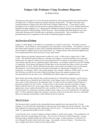
Figure 3. Example of a Weibull Plot.Interpreting a Weibull PlotThe Weibull plot can be a very powerful tool in making life predictions based on a set of data. Beforeproceeding further, however, it is necessary to define some terms. When evaluating fatigue data, theWeibull plot is the unreliability (U) of the population expressed as a function of life (x), U f(x). Life can beexpressed in terms of time, cycles, etc. The unreliability at any specified life is the fraction of thepopulation expected to fail before that life is achieved. Reliability (R) is the fraction of the populationexpected to survive at the specified life. The sum of the Reliability and Unreliability equals 1. In otherwords, the y-axis of the Weibull plot represents both U and 1-R.A very important and often misunderstood term related to Weibull analysis is confidence (C). Think ofconfidence as a measure of error in determining the Weibull parameters. By definition, the best-fit linethrough the data on the Weibull plot represents a confidence level of 50%. In other words, if additionaldata were collected from the same sample population used to generate a Weibull plot, the next data pointwould have a 50% chance of falling to the right side of the existing 50% Confidence line. An additionalinterpretation is demonstrated in the following example.Example 1.The Weibull plot shown in Figure 3 suggests 20% unreliability at a life of 90,426 cycles at aconfidence level of 50%. Assume a total of eight tests are to be conducted. The test apparatus isconfigured to test ten pieces simultaneously. It can be expected that in four of the tests (C 50%),more than two pieces will fail (U 20%) when testing reaches 90,426 cycles. In the remaining fourtests, it can be expected that less than two pieces will fail when testing reaches 90,426 cycles.Auxiliary curves can be constructed on the Weibull plot to represent different confidence levels. For agiven confidence level, the width of the band between the C 50% line and the new curve is a function ofthe number of data points in the data set. In other words, the more data used to calculate the distribution,the more certainty there is in the calculated results. Confidence levels greater than 50% are shown to theleft of the C 50% line while those lower than 50% are shown to the right. Typically, confidence levelsbelow 50% are not considered in the spring industry. Figure 4 shows the 90% confidence band added tothe Weibull plot in Figure 3. Similar to the scenario presented above, assume that additional data werecollected from the same sample population used to generate the plot in Figure 3. The next data point would