Transcription
Seagull: An Infrastructure for Load Prediction andOptimized Resource AllocationOlga Poppe, Tayo Amuneke, Dalitso Banda, Aritra De, Ari Green, Manon Knoertzer, EhiNosakhare, Karthik Rajendran, Deepak Shankargouda, Meina Wang, Alan Au, Carlo Curino, QunGuo, Alekh Jindal, Ajay Kalhan, Morgan Oslake, Sonia Parchani, Vijay Ramani, Raj Sellappan,Saikat Sen, Sheetal Shrotri, Soundararajan Srinivasan, Ping Xia, Shize Xu, Alicia Yang, Yiwen ZhuMicrosoft, One Microsoft Way, Redmond, WA 98052firstname.lastname@microsoft.comper week and manually sets the backup window during low customer activity. However, this solution is neither scalable to millionsof customers, nor durable since customer activity varies over time.More recently, customers can select a backup window themselves.However, they may not know the best time to run a backup. Insteadof these manual solutions, DS techniques could be deployed to predict customer load. These predictions could then be leveraged toschedule backups during expected low customer activity.An infrastructure that analyses historical load per system component, predicts its future load, and leverages these predictions tooptimize resource allocation is valuable for many products and usecases. Over the last two years we have built such an infrastructure,called Seagull, and applied it to two scenarios: (1) Backup scheduling of PostgreSQL and MySQL servers and (2) Preemptive auto-scaleof SQL databases. These scenarios required us to battle-test the infrastructure across all Azure regions and gave us confidence on thehigh impact and generality of the Seagull approach.Challenges. While building the Seagull infrastructure, we tackled the following open challenges. Design of an end-to-end infrastructure that predicts resourceutilization and leverages these predictions to optimize resourceallocation. This infrastructure must be: (a) Reusable for variousscenarios and (b) Scalable to millions of customers worldwide. Implementation and deployment of this infrastructure to production to predict customer activity and schedule backups such thatthey do not interfere with customer load. Accurate yet efficient customer low load prediction for optimizedbackup scheduling. This challenge includes choice of an ML modelthat finds the middle ground between accuracy and scalability. Inaddition, prediction accuracy must be redefined to focus on predicting the lowest valley in customer CPU load that is long enoughto fit a full backup of a server of its backup day. Accurate loadprediction for the whole day is less critical for backup scheduling.State-of-the-Art Approaches. Most of existing systems forML lack easy integration with Azure compute [8, 11, 15, 16, 23, 28].Thus, we built our solution based on Azure ML [4].While time series forecast in general and load prediction inparticular are well studied topics, none of the state-of-the-art approaches focused on predicting the lowest valley in customer CPUload for optimized backup scheduling. Instead, existing approachesfocus on, for example, idle time detection for predictive resourceprovisioning [26, 38], VM workload prediction for dynamic VMallocation [13, 14], and demand-driven auto-scale [18–22, 35, 36].Thus, these approaches do not tackle the unique challenges of lowABSTRACTMicrosoft Azure is dedicated to guarantee high quality of serviceto its customers, in particular, during periods of high customeractivity, while controlling cost. We employ a Data Science (DS)driven solution to predict user load and leverage these predictionsto optimize resource allocation. To this end, we built the Seagullinfrastructure that processes per-server telemetry, validates thedata, trains and deploys ML models. The models are used to predict customer load per server (24h into the future), and optimizeservice operations. Seagull continually re-evaluates accuracy ofpredictions, fallback to previously known good models and triggersalerts as appropriate. We deployed this infrastructure in production for PostgreSQL and MySQL servers across all Azure regions,and applied it to the problem of scheduling server backups duringlow-load time. This minimizes interference with user-induced loadand improves customer experience.PVLDB Reference Format:Poppe et al. Seagull: An Infrastructure for Load Prediction and OptimizedResource Allocation. PVLDB, 14(2): 154 - 162, osoft Azure, Google Cloud Platform, Amazon Web Services,and Rackspace Cloud Servers are the leading cloud service providersthat aim to guarantee high quality of service to their customers,while controlling operating costs [27, 38]. Achieving these conflicting goals manually is labor-intensive, time-consuming, error-prone,neither scalable, nor durable. Thus, these providers shift towardsautomatically managed services. To this end, Data Science (DS)techniques are deployed to predict resource demand and leveragethese predictions to optimize resource allocation [14].Motivation. Backups of databases are currently scheduled byan automated workflow that does not take typical customer activitypatterns into account. Thus, backups often collide with peaks ofcustomer activity resulting in inevitable competition for resourcesand poor quality of service during backup windows. To solve thisproblem currently, an engineer plots the customer load per databaseThis work is licensed under the Creative Commons BY-NC-ND 4.0 InternationalLicense. Visit https://creativecommons.org/licenses/by-nc-nd/4.0/ to view a copy ofthis license. For any use beyond those covered by this license, obtain permission byemailing info@vldb.org. Copyright is held by the owner/author(s). Publication rightslicensed to the VLDB Endowment.Proceedings of the VLDB Endowment, Vol. 14, No. 2 ISSN 2150-8097.doi:10.14778/3425879.3425886154
recognized by persistent forecast. We compared these models withrespect to accuracy and scalability on real production data duringone month in four Azure regions. Surprisingly, the accuracy of MLmodels is not significantly higher than the accuracy of persistentforecast. Thus, we deployed persistent forecast based on previousday to predict low load for all servers.Outline. We present the Seagull infrastructure in Section 2.We classify the servers in Section 3. Section 4 defines low load prediction accuracy. Section 5 compares the ML models. We evaluateSeagull in Sections 6, summarize lessons learned in Section 7 and,review related work in Section 8. Section 9 concludes the paper.2SEAGULL INFRASTRUCTUREIn this section, we summarize our design principles, give an overviewof the Seagull infrastructure, and describe how to reuse it.Figure 1: Seagull infrastructure2.1load prediction for optimized backup scheduling described above. Inparticular, they neither define the accuracy of low load prediction,nor compare several ML models with respect to low load prediction.Proposed Solution. We built the Seagull infrastructure (Figure 1) that deploys DS techniques to predict resource utilization andleverages these predictions to optimize resource allocation. Thisinfrastructure consumes prior load, validates this data, extracts features, trains an ML model, deploys this model to a REST endpoint,tracks the versions of all deployed models, predicts future load, andevaluates the accuracy of these predictions. We deployed Seagullto production worldwide to schedule backups of PostgreSQL andMySQL servers during time intervals of expected low customeractivity. We achieved several hundred hours of improved customerexperience across all regions per month.Contributions. Seagull features the following innovations. We designed and implemented an end-to-end Seagull infrastructure and deployed it in all Azure regions to optimize backupscheduling of PostgreSQL and MySQL servers. We describe ourdesign principles and lessons learned. We present our optimizationtechniques that reduce runtime and ensure scalability. We explainhow to reuse the infrastructure for other scenarios. We evaluate theimpact of the Seagull infrastructure on both improving customerexperience and reducing engineering effort. We conducted comprehensive analysis to classify the serversinto homogeneous groups based on their typical customer activitypatterns. Majority of servers are either stable or follow a daily or aweekly pattern. Thus, the load per server on previous (equivalent)day is a strong predictor of the load per server today. This heuristic, called persistent forecast, correctly predicted the lowest loadwindow per server on its backup day in 96% of cases. We defined the accuracy of low load window prediction asthe combination of two metrics. One, the lowest load window ischosen correctly if there is no other window that is long enough tofit a full backup and has significantly lower average user CPU load.Two, the load during a lowest load window is predicted accuratelyif majority of predicted data points are within a tight acceptableerror bound of their respective true data points. We applied several ML models commonly used for time seriesprediction (NimbusML [9], GluonTS [7], and Prophet [10]) to predictlow load of unstable servers that do not follow a pattern that can beDesign PrinciplesModularity. With the goal to reuse the Seagull infrastructurefor various products and scenarios at Microsoft, we had to designit in a modular way. At the same time, we were determined tosolve a specific task of optimized backup scheduling. To achieveboth goals, we grouped the use-case-agnostic and use-case-specificcomponents together (Figure 1). The use-case-agnostic componentscan be reused in several scenarios (Section 2.4). For example, anyML model can be plugged in. Nevertheless, the use-case-agnosticcomponents often have to be adjusted to a particular data set, product, and scenario. For example, if the load of most servers is stableor conforms to a business pattern (Section 3), a simple heuristiccan be used to predict the load. Complex ML models may not beneeded (Section 5). However, the usage patterns may change overtime. This observation justifies the need for a robust infrastructurethat automatically detects these changes, notifies about them, andallows to easily replace the model.Scalability. With the goal to deploy the Seagull infrastructurein all Azure regions, we had to ensure that it scales well for production data. Thus, we broke the input data down by region andran a DS pipeline per region. Since the size of regions varies, thesize of input files ranges from hundreds of kilobytes to a few gigabytes. Consequently, the runtime of a pipeline ranges from fewminutes to few hours (Figures 7(a) and 8). We used Dask [6] to runtime-consuming computations in parallel and achieved up to 4Xspeed-up compared to single-threaded execution (Figure 8(b)).The choice of an ML model is determined not only by its accuracybut also by its scalability. For example, ARIMA [2] is computationally intensive since it searches the optimal values of six parametersto make an accurate load prediction per server. Parameter sharingamong servers caused worsening of accuracy. While inference timeis within a few seconds, fitting may take up to 3 hours per server.Hence, executing ARIMA in parallel for each server does not makeruntime of ARIMA comparable to other models (Figure 7(a)). Thus,we excluded ARIMA from further consideration.2.2Use-Case-Agnostic Offline ComponentsThe use-case-agnostic components consume the load per systemcomponent (e.g., database, server, VM) and apply ML models topredict future load of this component.155
Load Extraction Module is implemented as a recurring querythat extracts relevant data from raw production telemetry andstores this data in Azure Data Lake Store (ADLS) [3]. These filesare input to the Azure ML pipeline.For the backup scheduling scenario, we have selected the averagecustomer CPU load percentage per five minutes as an indicator ofcustomer activity. Other signals (memory, I/O, number of activeconnections, etc.) can be added to improve accuracy. In this paper,customer CPU load percentage per server is referred to as load perserver for readability. Servers are due for full backup at least once aweek. Thus, the load extraction query runs once a week per region.Azure ML Pipeline is the core component of the Seagull infrastructure. It is built using the functionality of Azure MachineLearning (AML) [4] that facilitates end-to-end machine learninglife cycle. This pipeline consumes the load, validates it, extractsfeatures, trains a model, deploys the model, and makes it accessible through a REST endpoint. The pipeline tracks the versions ofdeployed models, performs inference, and evaluates the accuracyof predictions. Results are stored in Cosmos DB [5], globally distributed and highly available database service. Based on predictedload, resource allocation can be optimized in various ways.In our case, the predictions are input to the backup schedulingalgorithm. A run of the AML pipeline is scheduled once a weekper region since servers are due for full backup at least once aweek. Due to space limitations, we focus on the following five mostinteresting modules of the pipeline: Data Validation Module. Since data validation is a wellstudied topic [12], we implemented existing rules such as detectionof schema and bound anomalies. Feature Extraction Module. Lifespan and typical resourceusage patterns are features that are useful for load prediction. In particular, we differentiate between short-lived and long-lived servers,stable and unstable servers, servers that follow a daily or a weeklypattern and servers that do not conform to such a pattern, predictable and unpredictable servers in Sections 3 and 4.2. We willextend this module by other features [32] to improve accuracy. Model Training and Inference Modules. While many MLmodels can be plugged into the Seagull infrastructure, we compared NimbusML [9], GluonTS [7], and Prophet [10] with respectto accuracy and scalability. We applied these models to servers thatcannot be accurately predicted by persistent forecast in Section 5. Accuracy Evaluation Module. For backup scheduling, accurate load prediction for the whole day per server is less importantthan accurate prediction of lowest load window per day and server.Thus, we tailor prediction accuracy to our use case. We measure ifthe lowest load window is chosen correctly and if the load duringthis window is predicted accurately in Sections 3.1 and 4.Application Insights Dashboard [1] provides summarizedview of the pipeline runs to facilitate real-time monitoring andincident management. Examples of incidents include missing orinvalid input data, errors or exceptions in any step of the pipeline.2.3deploys executables which probe their respective services resultingin measurement of availability and quality of service. The runnerservice is deployed in each Azure region.For those servers that are due for full backups the next day, thebackup scheduling algorithm verifies if these servers were predictedcorrectly for the last three weeks. In this way, we verify that theservers were predictable for several weeks and we do not reschedulea backup at a worse time based on predictions we are not confidentin. Three weeks of history is a compromise between predictionconfidence and relevance of this rule to the majority of servers(58% of servers survive beyond three weeks, Figure 3). For suchpredictable servers, the algorithm extracts the predicted load forthe next day and selects a time window during which customeractivity is expected to be the lowest. The algorithm stores thestart time of this window as a service fabric property of respectivePostgreSQL and MySQL database instances. This property is usedby the backup service to schedule backups. Servers that did notexist or were unpredictable for the last three weeks are scheduledfor backup at default time.2.4Reuse of Seagull for Other ScenariosSo far, we applied the Seagull infrastructure to two different scenarios: (1) Backup scheduling of PostgreSQL and MySQL serversand (2) Preemptive auto-scale of SQL databases. Based on this experience, we now summarize how to reuse the use-case-agnosticcomponents of Seagull.No Changes. All interfaces between the use-case-agnostic components, Model Deployment and Tracking are designed independently from any scenario and require no changes.Parameter Updates. Data Ingestion and Validation, storage ofresults to CosmosDB, Pipeline Scheduler, Incident Management,and Application Insights Dashboard are parameterized to facilitateeasy adjustment to a new scenario. For example, to account forchanges of input data, we automatically deduce schema and otherdata properties (e.g., range of numeric attribute values) from theinput data. The schema and data properties are stored in a file. Afterthe file has been verified by a domain expert, it is used to detectschema and bound anomalies.Other components require similar parameter updates. For example, Data Ingestion requires update of the location of input data inADLS and access rights to this data. Also, the schema of CosmosDBtables, frequency of pipeline runs, and gathered statistics may bedifferent for other scenarios.Adjustments. Load Extraction, Feature Extraction, Model Training, Inference, and Accuracy Evaluation may require non-trivialcustomization. For example, other forecast signals (CPU, memory,disk, I/O, etc.) and features (subscriber identifier, number of activeconnections, etc.) may be needed for other scenarios. Accuracyand scalability of ML models heavily depend on the input data andscenario (Sections 3 and 5). Accuracy Evaluation may have to betailored to the use case requirements (Section 4).Use-Case-Specific Online Components3The use-case-specific components leverage predicted load to optimize backup scheduling. The backup scheduler runs within MasterData Service (MDS) runner per day and cluster. The Runner ServicePOSTGRESQL AND MYSQL SERVERSIn this section, we first define load prediction accuracy metric andthen use this metric to measure if a server has stable load or followsa daily or a weekly pattern.156
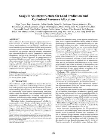
Figure 3: Classification of serversthousands of servers from four regions during one month in 2019,Figure 3 summarizes the percentage of servers per class.Figure 2: Acceptable error bound3.1Definition 3.3. (Short-Lived Server) A server is called long-livedif it existed more than three weeks. Otherwise, a server is calledshort-lived.Load Prediction Accuracy MetricWhile there are several established statistical measures of predictionerror (e.g., mean absolute scaled error and mean normalized rootmean squared error), we found them unintuitive and cumbersometo use in our case. They produce a number representing predictionerror per server per day. They give no insights into whether thelowest load window was chosen correctly per server per day norwhether the load was predicted accurately during this window.Thus, Definitions 3.2 and 4.2 below define these two metrics.As shown in Figure 3, 58% of servers survive for more thanthree weeks creating enough history to make a reliable conclusionwhether they are predictable (Section 4.2). Remaining 42% of serversare short-lived. We exclude them from further consideration.Definition 3.4. (Stable Server) A long-lived server is called stableduring a time interval 𝑡 if its load is accurately predicted by itsaverage load during the time interval 𝑡 (Definition 3.2). Otherwise,a server is called unstable.Definition 3.1. (Acceptable Error Bound, Bucket Ratio Metric) Given predicted and true load for a server 𝑠 during a timeinterval 𝑡, we define the bucket ratio metric for the server 𝑠 and theinterval 𝑡 as the percentage of predicted data points that are withinthe acceptable error bound of 10/ 5 of their respective true datapoints during 𝑡.53.5% of servers are long-lived and stable and thus easily predictable (Figure 3). 4.4% of long-lived unstable servers require amore detailed analysis. They are further classified into those thatfollow a daily or a weekly pattern and those that do not conformto such a pattern.Definition 3.1 specifies an asymmetric error bound that toleratesup to 10% over-predicted load but only at most 5% under-predictedload because a slight overestimation of low load periods is lesscritical for our use case than a slight underestimation that mayresult in interference with high customer load. In Definitions 3.1–4.3, we plug in constants that were empirically chosen by domainexperts and are now used in production for the backup schedulinguse case. Other constants can be plugged in for other scenarios.Definition 3.5. (Server with Daily Pattern) Given the load ofa server 𝑠 on two consecutive days 𝑑 1 and 𝑑, the server 𝑠 has adaily pattern on day 𝑑 if its load on day 𝑑 is accurately predictedby its load on the previous day 𝑑 1. A server has a daily patternduring a time interval 𝑡 if its load conforms to this daily pattern oneach day during the whole time period 𝑡.Figure 4 shows an example of a server with a strong daily pattern.We plot the load on this day in black and on the previous day inblue. These lines overlap almost perfectly. The bucket ratio is 95%.Such a precise daily pattern could be the result of an automatedrecurring workload.Definition 3.2. (Accurate Load Prediction) Prediction of theload of a server 𝑠 during a time interval 𝑡 is accurate if the bucketratio of the server 𝑠 during the time interval 𝑡 is at least 90%. Otherwise, a prediction is inaccurate.Definition 3.6. (Server with Weekly Pattern) Given the loadof a server 𝑠 on two consecutive equivalent days of the week 𝑑 7and 𝑑, the server 𝑠 has a weekly pattern on day 𝑑 if its load on day 𝑑is accurately predicted by its load on the previous equivalent day ofthe week 𝑑 7. A server has a weekly pattern during a time interval𝑡 if it does not have a daily pattern during the time period 𝑡 and itsload conforms to a weekly pattern on each day during the wholetime interval 𝑡.In Figure 2, we depict predicted load as blue line, true load asback line, and acceptable error bound as gray area. Intuitively, aprediction is accurate if 90% of the blue line is in the gray area. Eventhough the prediction looks close enough, the bucket ratio is only75%. Thus, this prediction is inaccurate. This example illustratesthat Definitions 3.1 and 3.2 impose strict constraints on accuracy.3.2Server ClassificationFigure 5 shows an example of a server that follows a weeklypattern. Similarly to previous Sunday (December 1), the load onthis Sunday (December 8) is medium before noon and high afternoon. The bucket ratio is over 90%. In contrast, the load on previousday (December 7) is low before noon and medium after noon. TheWe classify the servers with respect to typical customer behaviorin Figure 3. The classification provides valuable insights about loadpredictability. We will leverage these insights while choosing theML model in Section 5. Given a random sample of several tens of157
Figure 4: Server with daily patternFigure 6: Correctly chosen LL windowof full backup of the server 𝑠. True LL window for the server 𝑠 on theday 𝑑 is the time interval of length 𝑏 during which the average trueload of the server 𝑠 on the day 𝑑 is minimal across all other timeintervals of length 𝑏 on the day 𝑑. Predicted LL window is definedanalogously based on predicted load of the server 𝑠 on day 𝑑.Definition 4.2. (Correctly Chosen LL Window) Let 𝑤𝑡 and 𝑤 𝑝be the true and predicted LL windows for a server 𝑠 on day 𝑑. If theaverage true load during the predicted LL window 𝑤 𝑝 is within anacceptable error bound of the average true load during the true LLwindow 𝑤𝑡 , then the predicted LL window 𝑤 𝑝 is chosen correctly.In Figure 6, the true and predicted LL windows do not overlap.However, the average true load during true LL window is onlyslightly lower than the average true load during predicted LL window. Thus, the true LL window would not be a significantly bettertime interval to run a backup than the predicted LL window. Hence,we conclude that the predicted LL window is chosen correctly.Figure 5: Server with weekly patternbucket ratio is only 1%. Thus, we conclude that this server followsa weekly pattern but does not conform to a daily pattern.0.2% of servers conform to a daily or a weekly pattern and thusare easy to predict (Figure 3). Even though this percentage is relatively low, hundreds of top-revenue customers fall into this class ofservers and cannot be disregarded.Summary. Figure 3 illustrates that 53.7% of servers is expectedto be predictable because their load is either stable or conforms toa pattern. 4.2% of the servers are neither stable nor follow a pattern.They are likely to be unpredictable. 42.1% are short-lived and thusexcluded. These insights will be used while choosing the ML modelto predict low load per server in Section 5.44.2LOW LOAD PREDICTION ACCURACYIn addition to the load prediction accuracy metric in Section 3.1,we define the lowest load window metric. Based on these metrics,we formulate the backup scheduling problem.4.1Backup Scheduling Problem StatementFor each server 𝑠 that is due for full backup on day 𝑑, we aim to:(1) Correctly choose the LL window on day 𝑑 to schedule a backupduring this LL window on day 𝑑 and (2) Accurately predict theload during this LL window to move a backup from default backupday to another day of the week if the load is lower on another day.These two metrics are orthogonal. Indeed, the true and predicted LLwindows may coincide. However, the true load may be significantlyhigher than the predicted load [33]. The opposite case is also possible. Namely, the load may be predicted accurately during predictedLL window but the true load during the true LL window may bemuch lower than during the predicted LL window [33]. Based onthese observations, we conclude that only both metrics combinedgive us reliable insights about low load prediction accuracy.Lowest Load Window MetricDefinition 4.3. (Predictable Server) A long-lived server is calledpredictable if for the last three weeks its LL windows were chosencorrectly and the load during these windows was predicted accurately (Definitions 3.2 and 4.2).For each server on its backup day, our goal is to predict the lowestvalley in the user load that is long enough to run a full backupof this server. The time interval of this valley is called the lowestload window. We measure if this window is chosen correctly and ifthe load during this window is predicted accurately. Accurate loadprediction during the whole day is less critical in our case.As explained in Section 2, we change backup window for predictable servers only. Servers that did not exist or were not predictable for three weeks, default to current backup time that ischosen independently from customer activity.Definition 4.1. (Lowest Load (LL) Window) Let 𝑠 be a serverwhich is due for full backup on day 𝑑. Let 𝑏 be the expected duration158
(a) Training and inference(b) LL windows(c) Load during LL windows(d) Predictable serversFigure 7: Low load prediction using Persistent Forecast (PF), NimbusML (N), GluonTS (G), and Prophet (P)5the load of stable servers (Definition 3.4); 53.5% of servers are stable(Figure 3). Previous equivalent day is more powerful than previousweek average because it captures a weekly pattern (Definition 3.6),including stable load which covers 53.6% of servers. Previous day isalso more powerful than previous week average, since it captures adaily pattern (Definition 3.5), including stable load. 53.7% of serverscan be predicted by the previous day’s pattern. Since previous dayis suitable for the largest subset of servers, we focus on this variantin the following. Unstable servers that do not conform to a pattern that can be recognized by persistent forecast. 4.2% of servers fall into this category.In Section 5.3, we apply ML models to such servers to find out ifthese models can detect a predictable load pattern for these servers.LOW LOAD PREDICTIONIn this section, we describe the ML models commonly used fortime series forecast, choose a model per each class of servers, andcompare the models with respect to their accuracy and scalability.5.1ML Models for Time Series ForecastWe now summarize the key ideas of the ML models that we considered to predict low customer activity.Persistent Forecast refers to replicating previously seen loadper server as the forecast of the load for this server. We comparedthree variations of persistent forecast: Previous day takes the load per server on the previous day andutilizes it as predicted load on the next day. Previous equivalent day forecasts the load of a server by replicating its load on previous equivalent day of the week. Previous week average uses the average load per server duringprevious week as predicted load per server.NimbusML [9] is a Python module that provides Python bindings for ML.NET. NimbusML aims to enable data science teams thatare more familiar with Python to take advantage of ML.NET’s functionality and performance. It provides battle-tested, state-of-the-artML algorithms, transforms, and components. Specifically, we useSingular Spectrum Analysis to transform forecasts.GluonTS [7] is a toolkit for probabilistic time series modeling,focusing on deep learning-based models. We train a simple feedforward estimator. We tried several other estimators but this modelachieved highest accuracy.Prophet [10] is open source software released by Facebook.It forecasts a time series data based on an additive model wherenon-linear trends are fit with yearly, weekly, and daily seasonality,plus holiday effects. It works well for time series that have strongseasonal effects and several seasons of historical data. Prophet isrobust to missing data and shifts in the trend. It handles outlierswell. We fit Prophet with daily seasonality enabled.5.25.3Experimental Comparison of ML Models5.3.1 Experimental Setup. We conducted all experiments on a VMrunnin
weekly pattern. Thus, the load per server on previous (equivalent) day is a strong predictor of the load per server today. This heuris-tic, called persistent forecast, correctly predicted the lowest load window per server on its backup day in 96% of cases. We defined the accuracy of low load window prediction as the combination of two metrics.