WIXLIB

Distortion mapping correction in aspheric null testingM. Novak, C. Zhao, J. H. BurgeCollege of Optical Sciences, 1630 East University Boulevard, Tucson, AZ, 85721ABSTRACTWe describe methods to correct both symmetric and asymmetric distortion mapping errors induced by nulltesting elements such as holograms or null lenses. We show experimental results for direct measurementand correction of symmetric mapping distortion, as well as an example result for analytical mappingperformed using an orthogonal set of vector polynomials for asymmetric correction. The empiricaldetermination of symmetric distortion is made via calculation from predicted and measured changes toaberrations induced via known changes to the testing point.1. INTRODUCTIONAspheric primary mirrors are popular for astronomical telescope systems. These mirrors are polished toaspheric shapes to help minimize the overall length of the telescope system and provide additional opticalcorrection for improved telescope performance. Optical testing with high accuracy is necessary, from asearly a point in the fabrication process as is feasible, to efficiently converge to the proper finished opticalsurface. One potential obstacle encountered when fabricating aspheric surfaces is distortion present whenimaging through null elements in the optical test. Distortion arises due to imperfect imaging through a nulllens system and other optics in an interferometer or through a transmission CGH. The presence ofdistortion diminishes accuracy by mapping surface features to incorrect radial positions on the image plane.In this paper, we describe a method used to determine symmetric distortion which may prove practical forlarge asphere testing, as well as a more general correction method for asymmetric distortion. Thesetechniques can be used to enable efficient testing of aspheric optical surfaces.2. SYMMETRIC DISTORTIONIt is useful to know how much distortion is present in interferometric measurement data. The distortionmay arise not only from the distortion inherent to the null optics used in the asphere test, but also from thediverging and collimating optics as well as any internal optical elements in the interferometer. In thissection, we present a method to determine distortion applicable in cases of rotational symmetry in theimage of the part under test. We hope this method can provide an alternative efficient means ofdetermining distortion for correction of optical testing data.Interferometry XIV: Techniques and Analysis, edited by Joanna Schmit, Katherine Creath, Catherine E. Towers,Proc. of SPIE Vol. 7063, 706313, (2008) · 0277-786X/08/ 18 · doi: 10.1117/12.798151Proc. of SPIE Vol. 7063 706313-1

2.1 Determination via Aberration MonitoringTo illustrate, we first considered a hyperbolic lens tested against a perfect spherical surface. The layout isshown in the diagram in Figure 1.Figure 1. Hyperbolic lens and spherical return mirror.Consider that distortion present in such an optical system causes a mapping of mirror surface coordinates toa distorted coordinate frame in the image. This mapping is not at 1:1 from mirror surface to detector pixelcoordinates. Instead, the mapping can be written asρi mρ m (1 D ρ m2 ) ,(1)wherem 1, and D is the distortion expressed as percent/100.1 DIf a known focus shift is made in the optical test, we have a wavefront change that is expressed asWm ( ρ m ) Aρ m2 ,(2)which maps toWi ( ρ i ) A(1 2 D) ρ i 2 DAρ i .24(3)Here, A is the wavefront focus coefficient and D is the total linear distortion present in the imaging system(including the interferometer optics in addition to the null optics). We have ignored alignment errors inthis wavefront expression. A known amount of focus in the wavefront contributes focus and sphericalaberration to the measured result. By controlling wavefront focus and monitoring the resulting sphericalaberration, an estimate of the system distortion can be made.Once the distortion is determined, apolynomial transformation can be applied to remap the surface data appropriately.Proc. of SPIE Vol. 7063 706313-2

Figure 2 contains a plot of fourth order spherical aberration as a function of focus position in the optical testillustrated in Figure 1. These data can be used to write a set of equations relating wavefront coefficients forspherical (Z9) and focus (Z4) aberrations for individual measurement cases of varying defocus. This set ofequations can then be used to calculate wavefront coefficients in order to estimate the system distortion. Inpractice, we hope this technique will allow for estimation of the contribution of distortion that cannot bemodeled (i.e., distortion from imaging optics within the interferometric system used for testing that are ofunknown design or quality), for large aspheric surfaces where building an accurate fiducial mask may bechallenging as well as a safety risk to the surface.Figure 2. Plot of Z9 vs. test point shift for hyperbolic lens system2.2 Preliminary Experimental Result Based on This MethodTo show an example of this process, measurements were made to determine the distortion in the IR opticaltest of a 4.3 m hyperbolic primary mirror currently in fabrication in our facility. To check the truedistortion value, eight fiducial masks were placed on the mirror at known spacing and a map of themodulation was made to determine the image position of these fiducials relative to their actual mirrorposition. A photograph of the fiducials used for this traditional method of distortion determination isshown in Figure 3.Proc. of SPIE Vol. 7063 706313-3

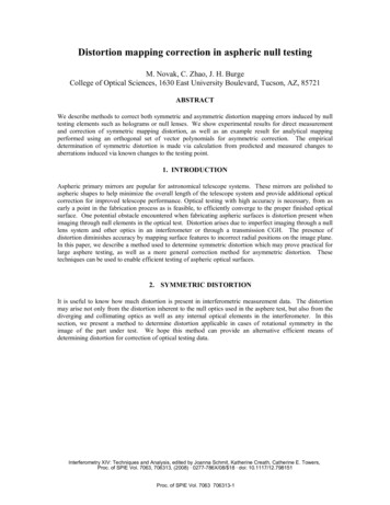
Figure 3. 4.3 m primary mirror with eight fiducial rings.Calculation based on these data provided an estimate of the distortion of the optical system ofapproximately –8% (D -0.08). The null lens was determined via modeling to have approximately -3.3%distortion; this indicates a significant distortion component is present in the interferometer optics. Afterthis initial determination of distortion, measurements were made of the optical surface, and aberrationswere monitored to keep track of the changing Zernike terms of interest (Z4 and Z9 for focus and sphericalaberration). Measured and predicted values of Z9 are plotted as a function of test point shift in Figure 4.Predicted and Measured Z9 vs. Test Point ShiftPredicted and Measured Z9 [microns]0.60000.4000Z9 (design/model) micronsZ9 measured [microns]0.20000.0000-6.0000 -5.0000 -4.0000 -3.0000 -2.0000 -1.0000 0.0000 1.0000 2.0000 3.0000 4.0000 5.0000-0.2000-0.4000-0.6000-0.8000Test Point Shift [mm]Figure 4. Z9 (predicted for null lens only and measured including total optical system) vs. test point shift for IRinterferometer measurement.These data indicate a slightly larger value of distortion present in the system than is indicated in thepredicted change with testing point. We consider this to be evidence of the distortion due to the internaloptical system of the interferometer. Calculation from these data gave distortion of -6.8% (D -0.068).Proc. of SPIE Vol. 7063 706313-4

The difference from the traditional correction may be attributed to limitations due to the imaging optics inour IR interferometer. Also, the instrument noise floor is not much lower than the values of sphericalaberration being measured in this case.3. ASYMMETRIC DISTORTIONIn this section, we describe a method used to correct asymmetric distortion in an optical null test. Webelieve this method can be applied in general cases where a transmission CGH test is used to fabricate offaxis aspheric surfaces; the distortion in this case does not preserve rotational symmetry.3.1 Vector Polynomial Mapping CorrectionWe now present an example of a more general distortion correction based on vector polynomial coordinatemapping. For this example, we consider the testing of an off axis parabola segment using a CGH null usedin transmission. In this optical test, distortion from the CGH causes a highly irregular image which mustbe corrected to avoid major difficulties in accurately figuring the proper location on the optical surface.The image of the part under test is distorted asymmetrically as shown in Figure 5.Mapping distortion:Test opticyImagey’xx’Measured map:Figure 5. Points on a test optic and their corresponding location in the image, as well as an illustration of a distortedsurface map.The mapping relationship between the test optic and its distorted image is determined solely by the opticsin between. The mapping of radial coordinates can be described as:rrr Mapping (r ') ,rrwhere r defines a point on the test optic, (x, y); and r ' defines a point on the camera, (x’, y’).The following steps are taken to determine this mapping relationship:Proc. of SPIE Vol. 7063 706313-5

1.Pick a set of base functions to describe the mapping relations2.Obtain r and r’ for a series of points3.Fit coefficients for the base functions describing the mapping relations between coordinates.We developed a series of orthonormal vector polynomials over a unit circle based on the gradient ofZernike polynomials. Pictures of a set of 12 of these polynomials are shown in Table 1.rS4rS3rS6/7 / / 1 1,'//1111NN\IIIII/N\\ I I I II S11rS12rS131 \ \ 7/1\7N\\ \ I 1 1 11/7/1/ /N'IiarS100arS5irS2Table 1. First 12 vector polynomials plotted on a unit circle.Proc. of SPIE Vol. 7063 706313-6@1

These vector polynomials are excellent candidates for the base functions for describing the mappingrelations in an asymmetrically distorted optical test image. We have used these polynomials with success infitting the mapping relations for the null test of the off-axis parabola segment (whose distorted map isshown in Figure 5.).To obtain the r and r’ pairs, a mask with regularly distributed holes can be laid on the test optic and theholes can then be located on the camera. The mask is shown in Figure 6.SSSSSSSSSTS: : : : : :-: : : : :S S S S S S S S S S S 5 SSSSSSSSSSSSSS .1Figure 6. Fiducial mask with 1” diameter holes located on a grid of 10” spacing.Once the base functions have been chosen and data for the r and r’ pairs has been measured, fitting themapping relationship is straightforward. We have written Matlab code to fit the mapping coefficients via aleast squares method. The resulting corrected surface map is shown below in Figure 7.Figure 7. Surface map of the test optic, a distortion-corrected version of the one shown in Figure 1.Proc. of SPIE Vol. 7063 706313-7

4. CONCLUSIONWe have described a method for empirical determination of rotationally symmetric distortion and shownresults of an experimental determination of distortion made in this way. There was approximately 15%difference between this experimental result and the estimation of distortion based on a traditional fiducialbased calculation. We consider this to be a limitation due to the imaging and relay optics in the IRinterferometric measurement we are using at the current state of fabrication of the mirror. We have alsoshown an example of correction of asymmetric distortion based on an analytical vector polynomialmapping of test optic to image coordinates which works very well for the correction of non-rotationallysymmetric distortion in optical testing data. These methods can be used to provide accurate knowledge ofthe position of surface features in order to efficiently fabricate aspheric optical surfaces.REFERENCESL.A. Selberg, “Interferometer accuracy and precision” Metrology: Figure and Finish, B. Truax, Editor.Proceedings SPIE 749 8-18, 1987.J.H. Burge, “Advanced techniques for measuring primary mirrors for astronomical telescopes”, Ph.D.dissertation, 1993.C. Zhao, J. H. Burge, “An Orthonormal Series of Vector Polynomials in a Unit Circle, Part II”, Opt.Express 16, 6586-6591 (2008).C. Zhao, J. H. Burge, “An Orthonormal Series of Vector Polynomials in a Unit Circle, Part I”, Opt.Express 15, 18014-18024 (2007).Proc. of SPIE Vol. 7063 706313-8

aberration being measured in this case. 3. ASYMMETRIC DISTORTION In this section, we describe a method used to correct asymmetric distortion in an optical null test. We believe this method can be applied in general cases wh ere a transmission CGH test is used to fabricate off axis aspheric surfaces; the distortion in this ca se does not preserve rotational symmetry. 3.1 Vector Polynomial .