Transcription
8Principal Component and Factor AnalysisKeywordsAkaike Information Criterion (AIC) Anti-image Bartlett method BayesInformation Criterion (BIC) Communality Components Confirmatory factoranalysis Correlation residuals Covariance-based structural equationmodeling Cronbach’s alpha Eigenvalue Eigenvectors Exploratory factoranalysis Factor analysis Factor loading Factor rotation Factor scores Factor weights Factors Heywood cases Internal consistency reliability Kaiser criterion Kaiser–Meyer–Olkin criterion Latent root criterion Measure of sampling adequacy Oblimin rotation Orthogonal rotation Oblique rotation Parallel analysis Partial least squares structural equationmodeling Path diagram Principal axis factoring Principal components Principal component analysis Principal factor analysis Promax rotation Regression method Reliability analysis Scree plot Split-half reliability Structural equation modeling Test-retest reliability Uniqueness VarimaxrotationLearning ObjectivesAfter reading this chapter, you should understand:– The basics of principal component and factor analysis.– The principles of exploratory and confirmatory factor analysis.– Key terms, such as communality, eigenvalues, factor loadings, factor scores, anduniqueness.– What rotation is.– The principles of exploratory and confirmatory factor analysis.– How to determine whether data are suitable for carrying out an exploratoryfactor analysis.– How to interpret Stata principal component and factor analysis output.# Springer Nature Singapore Pte Ltd. 2018E. Mooi et al., Market Research, Springer Texts in Business and Economics,DOI 10.1007/978-981-10-5218-7 8265
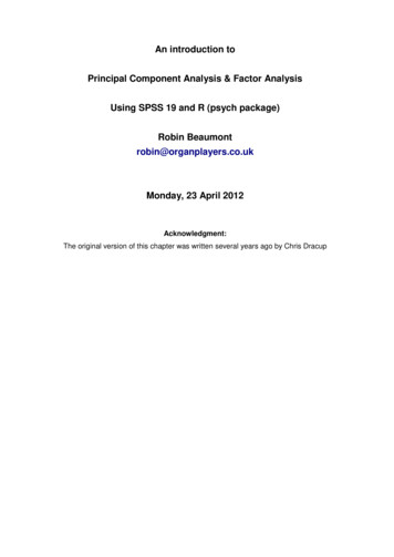
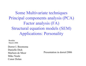
2668 Principal Component and Factor Analysis– The principles of reliability analysis and its execution in Stata.– The concept of structural equation modeling.8.1IntroductionPrincipal component analysis (PCA) and factor analysis (also called principalfactor analysis or principal axis factoring) are two methods for identifyingstructure within a set of variables. Many analyses involve large numbers ofvariables that are difficult to interpret. Using PCA or factor analysis helps findinterrelationships between variables (usually called items) to find a smaller numberof unifying variables called factors. Consider the example of a soccer club whosemanagement wants to measure the satisfaction of the fans. The management could,for instance, measure fan satisfaction by asking how satisfied the fans are with the(1) assortment of merchandise, (2) quality of merchandise, and (3) prices ofmerchandise. It is likely that these three items together measure satisfaction withthe merchandise. Through the application of PCA or factor analysis, we candetermine whether a single factor represents the three satisfaction items well.Practically, PCA and factor analysis are applied to understand much larger sets ofvariables, tens or even hundreds, when just reading the variables’ descriptions doesnot determine an obvious or immediate number of factors.PCA and factor analysis both explain patterns of correlations within a set ofobserved variables. That is, they identify sets of highly correlated variables andinfer an underlying factor structure. While PCA and factor analysis are very similarin the way they arrive at a solution, they differ fundamentally in their assumptionsof the variables’ nature and their treatment in the analysis. Due to these differences,the methods follow different research objectives, which dictate their areas ofapplication. While the PCA’s objective is to reproduce a data structure, as wellas possible only using a few factors, factor analysis aims to explain the variables’correlations by means of factors (e.g., Hair et al. 2013; Matsunaga 2010; Mulaik2009).1 We will discuss these differences and their implications in this chapter.Both PCA and factor analysis can be used for exploratory or confirmatorypurposes. What are exploratory and confirmatory factor analyses? Comparing theleft and right panels of Fig. 8.1 shows us the difference. Exploratory factoranalysis, often simply referred to as EFA, does not rely on previous ideas on thefactor structure we may find. That is, there may be relationships (indicated by thearrows) between each factor and each item. While some of these relationships maybe weak (indicated by the dotted arrows), others are more pronounced, suggestingthat these items represent an underlying factor well. The left panel of Fig. 8.1illustrates this point. Thus, an exploratory factor analysis reveals the number offactors and the items belonging to a specific factor. In a confirmatory factor1Other methods for carrying out factor analyses include, for example, unweighted least squares,generalized least squares, or maximum likelihood. However, these are statistically complex andinexperienced users should not consider them.
8.2Understanding Principal Component and Factor Analysis267Fig. 8.1 Exploratory factor analysis (left) and confirmatory factor analysis (right)analysis, usually simply referred to as CFA, there may only be relationshipsbetween a factor and specific items. In the right panel of Fig. 8.1, the first threeitems relate to factor 1, whereas the last two items relate to factor 2. Different fromthe exploratory factor analysis, in a confirmatory factor analysis, we have clearexpectations of the factor structure (e.g., because researchers have proposed a scalethat we want to adapt for our study) and we want to test for the expected structure.In this chapter, we primarily deal with exploratory factor analysis, as it conveysthe principles that underlie all factor analytic procedures and because the twotechniques are (almost) identical from a statistical point of view. Nevertheless,we will also discuss an important aspect of confirmatory factor analysis, namelyreliability analysis, which tests the consistency of a measurement scale (seeChap. 3). We will also briefly introduce a specific confirmatory factor analysisapproach called structural equation modeling (often simply referred to as SEM).Structural equation modeling differs statistically and practically from PCA andfactor analysis. It is not only used to evaluate how well observed variables relate tofactors but also to analyze hypothesized relationships between factors that theresearcher specifies prior to the analysis based on theory and logic.8.2Understanding Principal Component and Factor Analysis8.2.1Why Use Principal Component and Factor Analysis?Researchers often face the problem of large questionnaires comprising many items.For example, in a survey of a major German soccer club, the management wasparticularly interested in identifying and evaluating performance features that relateto soccer fans’ satisfaction (Sarstedt et al. 2014). Examples of relevant featuresinclude the stadium, the team composition and their success, the trainer, and the
2688 Principal Component and Factor AnalysisTable 8.1 Items in the soccer fan satisfaction studySatisfaction with. . .Condition of the stadiumInterior design of the stadiumOuter appearance of the stadiumSignposting outside the stadiumSignposting inside the stadiumRoofing inside the stadiumComfort of the seatsVideo score boards in the stadiumCondition of the restroomsTidiness within the stadiumSize of the stadiumView onto the playing fieldNumber of restroomsSponsors’ advertisements in the stadiumLocation of the stadiumName of the stadiumDetermination and commitment of the playersCurrent success regarding matchesIdentification of the players with the clubQuality of the team compositionPresence of a player with whom fans canidentifyPublic appearances of the playersNumber of stars in the teamInteraction of players with fansVolume of the loudspeakers in the stadiumChoice of music in the stadiumEntertainment program in the stadiumStadium speakerNewsmagazine of the stadiumPrice of annual season ticketEntry feesOffers of reduced ticketsDesign of the home jerseyDesign of the away jerseyAssortment of merchandiseQuality of merchandisePrices of merchandisePre-sale of ticketsOnline-shopOpening times of the fan-shopsAccessibility of the fan-shopsBehavior of the sales persons in the fanshopsmanagement. The club therefore commissioned a questionnaire comprising 99 previously identified items by means of literature databases and focus groups of fans.All the items were measured on scales ranging from 1 (“very dissatisfied”) to7 (“very satisfied”). Table 8.1 shows an overview of some items considered in thestudy.As you can imagine, tackling such a large set of items is problematic, because itprovides quite complex data. Given the task of identifying and evaluating performance features that relate to soccer fans’ satisfaction (measured by “Overall, howsatisfied are you with your soccer club”), we cannot simply compare the items on apairwise basis. It is far more reasonable to consider the factor structure first. Forexample, satisfaction with the condition of the stadium (x1), outer appearance of thestadium (x2), and interior design of the stadium (x3) cover similar aspects that relateto the respondents’ satisfaction with the stadium. If a soccer fan is generally verysatisfied with the stadium, he/she will most likely answer all three items positively.Conversely, if a respondent is generally dissatisfied with the stadium, he/she is mostlikely to be rather dissatisfied with all the performance aspects of the stadium, suchas the outer appearance and interior design. Consequently, these three items arelikely to be highly correlated—they cover related aspects of the respondents’overall satisfaction with the stadium. More precisely, these items can be interpreted
8.2Understanding Principal Component and Factor Analysis269as manifestations of the factor capturing the “joint meaning” of the items related toit. The arrows pointing from the factor to the items in Fig. 8.1 indicate this point. Inour example, the “joint meaning” of the three items could be described as satisfaction with the stadium, since the items represent somewhat different, yet related,aspects of the stadium. Likewise, there is a second factor that relates to the twoitems x4 and x5, which, like the first factor, shares a common meaning, namelysatisfaction with the merchandise.PCA and factor analysis are two statistical procedures that draw on itemcorrelations in order to find a small number of factors. Having conducted theanalysis, we can make use of few (uncorrelated) factors instead of many variables,thus significantly reducing the analysis’s complexity. For example, if we find sixfactors, we only need to consider six correlations between the factors and overallsatisfaction, which means that the recommendations will rely on six factors.8.2.2Analysis StepsLike any multivariate analysis method, PCA and factor analysis are subject tocertain requirements, which need to be met for the analysis to be meaningful. Acrucial requirement is that the variables need to exhibit a certain degree of correlation. In our example in Fig. 8.1, this is probably the case, as we expect increasedcorrelations between x1, x2, and x3, on the one hand, and between x4 and x5 on theother. Other items, such as x1 and x4, are probably somewhat correlated, but to alesser degree than the group of items x1, x2, and x3 and the pair x4 and x5. Severalmethods allow for testing whether the item correlations are sufficiently high.Both PCA and factor analysis strive to reduce the overall item set to a smaller setof factors. More precisely, PCA extracts factors such that they account forvariables’ variance, whereas factor analysis attempts to explain the correlationsbetween the variables. Whichever approach you apply, using only a few factorsinstead of many items reduces its precision, because the factors cannot represent allthe information included in the items. Consequently, there is a trade-off betweensimplicity and accuracy. In order to make the analysis as simple as possible, wewant to extract only a few factors. At the same time, we do not want to lose toomuch information by having too few factors. This trade-off has to be addressed inany PCA and factor analysis when deciding how many factors to extract fromthe data.Once the number of factors to retain from the data has been identified, we canproceed with the interpretation of the factor solution. This step requires us toproduce a label for each factor that best characterizes the joint meaning of all thevariables associated with it. This step is often challenging, but there are ways offacilitating the interpretation of the factor solution. Finally, we have to assess howwell the factors reproduce the data. This is done by examining the solution’sgoodness-of-fit, which completes the standard analysis. However, if we wish tocontinue using the results in further analyses, we need to calculate the factor scores.
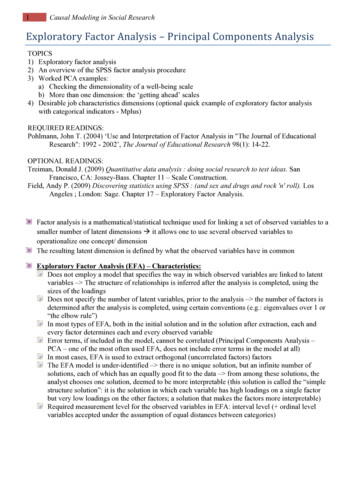
2708 Principal Component and Factor AnalysisFig. 8.2 Steps involved in a PCAFactor scores are linear combinations of the items and can be used as variables infollow-up analyses.Figure 8.2 illustrates the steps involved in the analysis; we will discuss these inmore detail in the following sections. In doing so, our theoretical descriptions willfocus on the PCA, as this method is easier to grasp. However, most of ourdescriptions also apply to factor analysis. Our illustration at the end of the chapteralso follows a PCA approach but uses a Stata command (factor, pcf), whichblends the PCA and factor analysis. This blending has several advantages, whichwe will discuss later in this chapter.8.3Principal Component Analysis8.3.1Check Requirements and Conduct Preliminary AnalysesBefore carrying out a PCA, we have to consider several requirements, which we cantest by answering the following questions:––––Are the measurement scales appropriate?Is the sample size sufficiently large?Are the observations independent?Are the variables sufficiently correlated?
8.3Principal Component Analysis271Are the measurement scales appropriate?For a PCA, it is best to have data measured on an interval or ratio scale. In practicalapplications, items measured on an ordinal scale level have become common.Ordinal scales can be used if:– the scale points are equidistant, which means that the difference in the wordingbetween scale steps is the same (see Chap. 3), and– there are five or more response categories.Is the sample size sufficiently large?Another point of concern is the sample size. As a rule of thumb, the number of(valid) observations should be at least ten times the number of items used foranalysis. This only provides a rough indication of the necessary sample size.Fortunately, researchers have conducted studies to determine minimum samplesize requirements, which depend on other aspects of the study. MacCallum et al.(1999) suggest the following:– When all communalities (we will discuss this term in Sect. 8.3.2.4) are above0.60, small sample sizes of below 100 are adequate.– With communalities around 0.50, sample sizes between 100 and 200 aresufficient.– When communalities are consistently low, with many or all under 0.50, a samplesize between 100 and 200 is adequate if the number of factors is small and eachof these is measured with six or more indicators.– When communalities are consistently low and the factors numbers are high orare measured with only few indicators (i.e., 3 or less), 300 observations arerecommended.Are the observations independent?We have to ensure that the observations are independent. This means that theobservations need to be completely unrelated (see Chap. 3). If we use dependentobservations, we would introduce “artificial” correlations, which are not due to anunderlying factor structure, but simply to the same respondents answered the samequestions multiple times.Are the variables sufficiently correlated?As indicated before, PCA is based on correlations between items. Consequently,conducting a PCA only makes sense if the items correlate sufficiently. The problemis deciding what “sufficient” actually means.An obvious step is to examine the correlation matrix (Chap. 5). Naturally, wewant the correlations between different items to be as high as possible, but theywill not always be. In our previous example, we expect high correlations betweenx1, x2, and x3, on the one hand, and x4 and x5 on the other. Conversely, we might
2728 Principal Component and Factor Analysisexpect lower correlations between, for example, x1 and x4 and between x3 and x5.Thus, not all of the correlation matrix’s elements need to have high values. ThePCA depends on the relative size of the correlations. Therefore, if singlecorrelations are very low, this is not necessarily problematic! Only when all thecorrelations are around zero is PCA no longer useful. In addition, the statisticalsignificance of each correlation coefficient helps decide whether it differs significantly from zero.There are additional measures to determine whether the items correlate sufficiently. One is the anti-image. The anti-image describes the portion of an item’svariance that is independent of another item in the analysis. Obviously, we want allitems to be highly correlated, so that the anti-images of an item set are as small aspossible. Initially, we do not interpret the anti-image values directly, but use ameasure based on the anti-image concept: The Kaiser–Meyer–Olkin (KMO)statistic. The KMO statistic, also called the measure of sampling adequacy(MSA), indicates whether the other variables in the dataset can explain thecorrelations between variables. Kaiser (1974), who introduced the statistic,recommends a set of distinctively labeled threshold values for KMO and MSA,which Table 8.2 presents.To summarize, the correlation matrix with the associated significance levelsprovides a first insight into the correlation structures. However, the final decision ofwhether the data are appropriate for PCA should be primarily based on the KMOstatistic. If this measure indicates sufficiently correlated variables, we can continuethe analysis of the results. If not, we should try to identify items that correlate onlyweakly with the remaining items and remove them. In Box 8.1, we discuss how todo this.Table 8.2 Thresholdvalues for KMO and MSAKMO/MSA valueBelow 90 and higherAdequacy of the eritoriousMarvelousBox 8.1 Identifying Problematic ItemsExamining the correlation matrix and the significance levels of correlationsallows identifying items that correlate only weakly with the remaining items.An even better approach is examining the variable-specific MSA values,which are interpreted like the overall KMO statistic (see Table 8.2). In fact,the KMO statistic is simply the overall mean of all variable-specific MSAvalues. Consequently, all the MSA values should also lie above the threshold(continued)
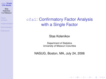
8.3Principal Component Analysis273Box 8.1 (continued)level of 0.50. If this is not the case, consider removing this item from theanalysis. An item’s communality or uniqueness (see next section) can alsoserve as a useful indicators of how well the factors extracted represent anitem. However, communalities and uniqueness are mostly considered whenevaluating the solution’s goodness-of-fit.8.3.2Extract the Factors8.3.2.1 Principal Component Analysis vs. Factor AnalysisFactor analysis assumes that each variable’s variance can be divided into commonvariance (i.e., variance shared with all the other variables in the analysis) andunique variance (Fig. 8.3), the latter of which can be further broken down intospecific variance (i.e., variance associated with only one specific variable) and errorvariance (i.e., variance due to measurement error). The method, however, can onlyreproduce common variance. Thereby factor analysis explicitly recognizes thepresence of error. Conversely, PCA assumes that all of each variable’s variance iscommon variance, which factor extraction can explain fully (e.g., Preacher andMacCallum 2003). These differences entail different interpretations of theanalysis’s outcomes. PCA asks:Which umbrella term can we use to summarize a set of variables that loads highly on aspecific factor?Conversely, factor analysis asks:What is the common reason for the strong correlations between a set of variables?From a theoretical perspective, the assumption that there is a unique variance forwhich the factors cannot fully account, is generally more realistic, but simultaneously more restrictive. Although theoretically sound, this restriction can sometimes lead to complications in the analysis, which have contributed to thewidespread use of PCA, especially in market research practice.Researchers usually suggest using PCA when data reduction is the primaryconcern; that is, when the focus is to extract a minimum number of factors thataccount for a maximum proportion of the variables’ total variance. In contrast, if theprimary concern is to identify latent dimensions represented in the variables, factoranalysis should be applied. However, prior research has shown that both approachesarrive at essentially the same result when:– more than 30 variables are used, or– most of the variables’ communalities exceed 0.60.
2748 Principal Component and Factor AnalysisFig. 8.3 Principal component analysis vs. factor analysisWith 20 or fewer variables and communalities below 0.40—which are clearlyundesirable in empirical research—the differences are probably pronounced(Stevens 2009).Apart from these conceptual differences in the variables’ nature, PCA and factoranalysis differ in the aim of their analysis. Whereas the goal of factor analysis is toexplain the correlations between the variables, PCA focuses on explaining thevariables’ variances. That is, the PCA’s objective is to determine the linearcombinations of the variables that retain as much information from the originalvariables as possible. Strictly speaking, PCA does not extract factors, butcomponents, which are labeled as such in Stata.Despite these differences, which have very little relevance in many commonresearch settings in practice, PCA and factor analysis have many points in common.For example, the methods follow very similar ways to arrive at a solution and theirinterpretations of statistical measures, such as KMO, eigenvalues, or factorloadings, are (almost) identical. In fact, Stata blends these two procedures in itsfactor, pcf command, which runs a factor analysis but rescales the estimatessuch that they conform to a PCA. That way, the analysis assumes that the entirevariance is common but produces (rotated) loadings (we will discuss factor rotationlater in this chapter), which facilitate the interpretation of the factors. In contrast, ifwe would run a standard PCA, Stata would only offer us eigenvectors whose(unrotated) weights would not allow for a concluding interpretation of the factors.In fact, in many PCA analyses, researchers are not interested in the interpretation ofthe extracted factors but merely use the method for data reduction. For example, insensory marketing research, researchers routinely use PCA to summarize a large setof sensory variables (e.g., haptic, smell, taste) to derive a set of factors whose scoresare then used as input for cluster analyses (Chap. 9). This approach allows foridentifying distinct groups of products from which one or more representativeproducts can then be chosen for a more detailed comparison using qualitative
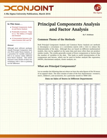
8.3Principal Component Analysis275research or further assessment in field experiments (e.g., Carbonell et al. 2008;Vigneau and Qannari 2002).Despite the small differences of PCA and factor analysis in most researchsettings, researchers have strong feelings about the choice of PCA or factoranalysis. Cliff (1987, p. 349) summarizes this issue well, by noting that proponentsof factor analysis “insist that components analysis is at best a common factoranalysis with some error added and at worst an unrecognizable hodgepodge ofthings from which nothing can be determined.” For further discussions on thistopic, see also Velicer and Jackson (1990) and Widaman (1993).28.3.2.2 How Does Factor Extraction Work?PCA’s objective is to reproduce a data structure with only a few factors. PCA doesthis by generating a new set of factors as linear composites of the original variables,which reproduces the original variables’ variance as best as possible. These linearcomposites are called principal components, but, for simplicity’s sake, we refer tothem as factors. More precisely, PCA computes eigenvectors. These eigenvectorsinclude so called factor weights, which extract the maximum possible variance ofall the variables, with successive factoring continuing until a significant share of thevariance is explained.Operationally, the first factor is extracted in such a way that it maximizes thevariance accounted for in the variables. We can visualize this easily by examiningthe vector space illustrated in Fig. 8.4. In this example, we have five variables (x1–x5) represented by five vectors starting at the zero point, with each vector’s lengthstandardized to one. To maximize the variance accounted for, the first factor F1 isfitted into this vector space in such a way that the sum of all the angles between thisfactor and the five variables in the vector space is minimized. We do this to interpretthe angle between two vectors as correlations. For example, if the factor’s vectorand a variable’s vector are congruent, the angle between these two is zero,Fig. 8.4 Factor extraction(Note that Fig. 8.4 describes aspecial case, as the fivevariables are scaled down intoa two-dimensional space. Inthis set-up, it would bepossible for the two factors toexplain all five items.However, in real-life, the fiveitems span a five-dimensionalvector space.)2Related discussions have been raised in structural equation modeling, where researchers haveheatedly discussed the strengths and limitations of factor-based and component-based approaches(e.g., Sarstedt et al. 2016, Hair et al. 2017a, b).
2768 Principal Component and Factor Analysisindicating that the factor and the variable correlate perfectly. On the other hand, ifthe factor and the variable are uncorrelated, the angle between these two is 90 . Thiscorrelation between a (unit-scaled) factor and a variable is called the factorloading. Note that factor weights and factor loadings essentially express the samething—the relationships between variables and factors—but they are based ondifferent scales.After extracting F1, a second factor (F2) is extracted, which maximizes theremaining variance accounted for. The second factor is fitted at a 90 angle intothe vector space (Fig. 8.4) and is therefore uncorrelated with the first factor.3 If weextract a third factor, it will explain the maximum amount of variance for whichfactors 1 and 2 have hitherto not accounted. This factor will also be fitted at a 90 angle to the first two factors, making it independent from the first two factors(we don’t illustrate this third factor in Fig. 8.4, as this is a three-dimensional space).The fact that the factors are uncorrelated is an important feature, as we can use themto replace many highly correlated variables in follow-up analyses. For example,using uncorrelated factors as independent variables in a regression analysis helpssolve potential collinearity issues (Chap. 7).The Explained Visually webpage offers an excellent illustration of two- andthree-dimensional factor extraction, see n important PCA feature is that it works with standardized variables (seeChap. 5 for an explanation of what standardized variables are). Standardizingvariables has important implications for our analysis in two respects. First, wecan assess each factor’s eigenvalue, which indicates how much a specific factorextracts all of the variables’ variance (see next section). Second, the standardizationof variables allows for assessing each variable’s communality, which describes howmuch the factors extracted capture or reproduce each variable’s variance. A relatedconcept is the uniqueness, which is 1–communality (see Sect. 8.3.2.4).8.3.2.3 What Are Eigenvalues?To understand the concept of eigenvalues, think of the soccer fan satisfaction study(Fig. 8.1). In this example, there are five variables. As all the variables arestandardized prior to the analysis, each has a variance of 1. In a simplified way,we could say that the overall information (i.e., variance) that we want to reproduceby means of factor extraction is 5 units. Let’s assume that we extract the two factorspresented above.The first factor’s eigenvalue indicates how much variance of the total variance(i.e., 5 units) this factor accounts for. If this factor has an eigenvalue of, let’s say3Note that this changes when oblique rotation is used. We will discuss factor rotation later in thischapter.
8.3Principal Component Analysis277Fig. 8.5 Total variance explained by variables and factors2.10, it covers the information of 2.10 variables or, put differently, accounts for2.10/5.00 ¼ 42% of the overall variance (Fig. 8.5).Extracting a second factor will allow us to explain another part of the remainingvariance (i.e., 5.00 – 2.10 ¼ 2.90 units, Fig. 8.5). However, the eigenvalue of thesecond factor will always be smaller than that of the first factor. Assume that thesecond factor has an eigenvalue of 1.30 units. The second factor then accounts for1.30/5.00 ¼ 26% of the overall variance. Together, these two factors explain(2.10 1.30)/5.00 ¼ 68% of the overall variance. Every additional factor extractedincreases the variance accounted for until we have extracted as many factors asthere are variables. In this case, the factors account for 100% of the overallvariance, which means that the factors reproduce the complete variance.Following
the exploratory factor analysis, in a confirmatory factor analysis, we have clear expectations of the factor structure (e.g., because researchers have proposed a scale that we want to adapt for our study) and we want to test for the expected structure. In this chapter, we primarily deal with exploratory factor analysis, as it conveys