WIXLIB

Factor analysis and Principal Component Analysis (PCA)3 Overview of the processThere are many varieties of factor analysis involving a multitude of different techniques, however the commoncharacteristic is that factor analysis is carried out using a computer although the early researchers in this areawere not so lucky, with the first paper introducing factor analysis being published in 1904 by C. Spearman ofSpearman’s rank correlation coefficient fame, long before the friendly PC was available.Factor analysis works only on interval/ratio data, and ordinal data at a push. If you want to carry out some typeof variable reduction process on nominal data you have to use other techniques or substantially adapt the factoranalysis see Bartholomew, Steele, Moustaki & Galbraith 2008 for details.3.1 Data preparationAny statistical analysis starts with standard data preparation techniques and factor analysis is no different. Basicdescriptive statistics are produced to note any missing/abnormal values and appropriate action taken. Also inaddition to this two other processes are undertaken:1. Any computed variables (slickly speaking only linear transformations) are excluded from the analysis.These are easily identified as they will have a correlation of 1 with the variable from which they werecalculated.2. All the variables should measure the construct in the same direction. Considering the GP satisfactionscale we need all the 14 items to measure satisfaction in the same direction where a score of 1represents high satisfaction and 5 the least satisfaction or the other way round. The direction does notmatter the important thing is that all the questions score in the same direction. Taking question 1: Mydoctor treats me in a friendly manner and question, this provides the value 1 when the respondentagrees, representing total satisfaction and 5 when the respondent strongly disagrees and is not satisfied.However question three is different: My doctor seems cold and impersonal. A patient indicating strongagreement to this statement would also provide a value of 1 but this time it indicates a high level ofdissatisfaction. The solution is to reverse score all these negatively stated questions.Considering our Holzinger and Swineford dataset we see that we have 73 cases and from the descriptive statisticsproduced earlier there appears no missing values and no out of range values. Also the correlation matrix does notcontain any ‘1’’s except the expected diagonals.3.2 Do we have appropriate correlations to carry out the factor analysis?The starting point for all factor analysis techniques is the correlation matrix. All factor analysis techniques try toclump subgroups of variables togetherbased upon their correlations and oftenyou can get a feel for what the factorsare going to be just by looking at thecorrelation matrix and spotting clustersof high correlations between groups ofvariables.Looking at the matrix from the Holzingerand Swineford dataset we see thatWordmean, sentence and paragraphseem to form one cluster and lozenges,cubes and visperc tests the other cluster.Norman and Streiner (p 197) quote Tabachnick & Fidell (2001) saying that if there are few correlations above 0.3it is a waste of time carrying on with the analysis, clearly we do not have that problem.Besides looking at the correlations we can also consider any number of other matrixes that the various statisticalcomputer programs produce. I have listed some below and filled in some details.C:\temporary from virtualclassroom\pca1.docxPage 6 of 24

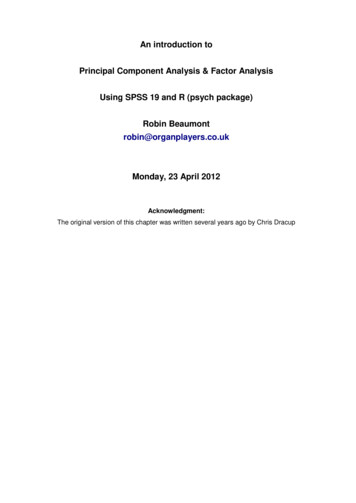
Factor analysis and Principal Component Analysis (PCA)Exercise 2.Considering each of the following matrixes complete the table below:Name of the matrixCorrelation ‘R’Elements are:correlationsPartial correlationAnti-image correlationPartial correlations reversedGood signsMany above 0.3 andpossible clusteringFew above 0.3 andpossible clusteringFew above 0.3 andpossible clusteringBad signsFew above 0.3Many above 0.3Many above 0.3While eyeballing is a valid method of statistical analysis (!) obviously some type of statistic, preferably with anassociated probability density function to produce a p value, would be useful to help us make this decision. Twosuch statistics are the Bartlett test of Sphericity and the Kaiser-Meyer-Olkin Measure of Sampling Adequacy(usually called the MSA).The Bartlett Test of Sphericity compares the correlation matrix with a matrix of zero correlations (technicallycalled the identity matrix, which consists of all zeros except the 1’s along the diagonal). From this test we arelooking for a small p value indicating that it is highly unlikely for us to have obtained the observed correlationmatrix from a population with zero correlation. However there are many problems with the test – a small pvalue indicates that you should not continue but a large p value does not guarantee that all is well (Norman &Streiner p 198).The MSA does not produce a P value but we are aiming for a value over 0.8 and below 0.5 is considered to bemiserable! Norman & Streiner p 198 recommend that you consider removing variables with a MSA below 0.7In SPSS we can obtain both the statistics by selecting the menu option Analyse- dimension reduction and thenplacing the variables in the variables dialog box and then selectingthe descriptives button and selecting the Anti-image option to showthe MSA for each variable and the KMO and Bartlett’s test for theoverall MSA as well:KMO and Bartlett's TestKaiser-Meyer-Olkin Measure of Sampling Adequacy.Approx. Chi-SquareBartlett's Test of age -.015-.209-.486a. Measures of Sampling -.176-.133.371.191-.015-.209-.486-.346.743aWe can see that we have good values forAnti-imageCorrelationall variables for the MSA but the overallvalue is a bit low at 0.763, howeverBartlett’s Test of Sphericity has anassociated P value (sig in the table) of 0.001 as by default SPSS reports p values of less than 0.001 as 0.000! So from the above results we know thatwe can now continue and perform a valid factor analysis.Finally I mentioned that we should exclude variables that are just simple derivations of another in the analysis,say variable A variable B 4. A similar problem occurs with variables that are very highly correlated (this iscalled multicollinearity) and when this occurs the computer takes a turn and can’t produce valid factor loadingvalues. A simple way of assessing this is to inspect a particular summary measure of the correlation matrix calledthe determinant and check to see if it is greater than 0.00001 (Field 2012 p771). Clicking on the determinantoption in the above dialog box produces a determinant value of 0.0737 for our dataset.C:\temporary from virtualclassroom\pca1.docxPage 7 of 24

Factor analysis and Principal Component Analysis (PCA)3.3 Extracting the FactorsThere are numerous ways to do this, and to get an idea you just need to look at the pull down list box in SPSSshown opposite.There are two common methods, the Principal components andthe Principal axis factoring extraction methods and strictlyspeaking the Principal components method is not a type of factoranalysis but it often gives very similar results. Let’s try both andsee what we get.However there is one other thing we need to consider first. Howmany latent variables do we want or do we want the computer todecide for use using some criteria – the common method is to letthe computer decide for use by simply selecting the Eigenvaluesgreater than 1 option however there are several reasons why thisis not an altogether good idea both Norman & Streiner 2008 and Field 2012 discuss them in detail. For now I’lluse the dodgy eigenvalue 1 approach.I have run both a Principal Axis and also a Principal Component Analysis below.Principal Axis (PA)Principal component (PCA)Factor an.778-.330Extraction Method: Principal Axis Factoring.a. 2 factors extracted. 11 iterations required.Component dmean.794-.427Extraction Method: Principal Component Analysis (PCA).a. 2 components 14Extraction Method: Principal Axis 50paragraph.826sentence.797wordmean.812Extraction Method: Principal Component Analysis.Total Variance ExplainedExtraction Sums of Squared LoadingsTotal% of VarianceCumulative action Method: Principal Axis Factoring.Total Variance ExplainedExtraction Sums of Squared LoadingsComponentTotal% of VarianceCumulative raction Method: Principal Component Analysis.FactorCommunalitiesYou will notice that both methods extracted 2 factors. However the factor loadings (or strictly speaking thecomponent loadings for the PCA) for the PCA are larger in absolute values as are the communalities and as aconsequence the total variance explained is also greater. Here are a few pointers to help you interpret the above:Factor loadings for the PA correlation between a specific observed variable and a specific factor. Higher valuesmean a closer relationship. They are equivalent to standardised regression coefficients (β weights) in multipleregression. Higher the value the better.Communality for the PA Is the total influence on a single observed variable from all the factors associated withit. It is equal to the sum of all the squared factor loadings for all the factors related to the observed variable andthis value is the same as R2 in multiple regression. The value ranges from zero to 1 where 1 indicates that thevariable can be fully defined by the factors and has no uniqueness. In contrast a value of 0 indicates that thevariable cannot be predicted at all from any of the factors. The communality can be derived for each variable bytaking the sum of the squared factor loadings for each of the factors associated with the variable. So for visperc 0.5552 0.4232 0.4869 and for cubes 0.4522 0.5532 0.510 These values can be interpreted the same way asR squared values in multiple regression that is they represent the % of variability attributed to the model,inspecting the total variance explained table in the above analyses you will notice that this is how the % ofC:\temporary from virtualclassroom\pca1.docxPage 8 of 24

Factor analysis and Principal Component Analysis (PCA)variance column is produced. Because we are hoping that the observed dataset is reflected in the model wewant this value to be as high as possible, nearer to one the better.Uniqueness for each observed variable it is that portion of the variable that cannot be predicted from the othervariables (i.e. the latent variables). It’s value is 1-communality. So for wordmean we have 1-0.714 0.286 and asthe communality can be interpreted as the % of the variablility that is predicted by the model we can say this isthe % variability in a specific observed variable that is NOT predicted by the model. This means that we want thisvalue for each observed variable to be as low as possible. On pgae 3 referring to the diagram it is the ‘error’arrow.Total variance explained this indicates how much of the variability in the data has been modelled by theextracted factors. You might think that given that the PCA analysis models 74% of the variability compared to just61% for the PA analysis we should go for the PCA results. However why the estimate is higher is because in thePCA analysis the initial estimates for the communalities are all set to 1 which is higher than for the PA analysiswhich uses an estimate of the R2 value also whereas the PCA makes use of all the variability available in thedataset in the PA analysis the unique variability for each observed variable is disregarded as we are only reallyinterested in how each relates to the latent variable(s). What is an acceptable level of variance explained by themodel? Well one would hope for the impossible which would be 100% often analyses are reported with 60-70%.Besides using the eigenvalue 1 criteria we could have inspected a scree pot and worked out where the factorslevelled off – we will look at this approach latter.Now we have our factors we need to find a way of interpreting them – to enable this wecarry out a process called factor rotation.3.4 Giving the factors meaningNorman & Streiner provide an excellent discussion as to the reasons for rotation ingiving factors meaning. To select a rotation method in SPSS you select the Rotationbutton in the factor analysis dialog box. We will consider two types Varimax andPromax. First Varimax:Varimax rotation from the PCA extraction methodRotated Component ean.891.137Extraction Method: Principal Component Analysis.Rotation Method: Varimax with Kaiser Normalization.a. Rotation converged in 3 iterations.Varimax rotation from the PA extraction methodRotated Factor .829.167Extraction Method: Principal Axis Factoring.Rotation Method: Varimax with Kaiser Normalization.a. Rotation converged in 3 iterations.We can seefrom both of the above set of results that they are prettysimilar. Paragraph, sentence and Wordmean load heavily onthe first factor/component and the other three on thesecond factor/component.By selecting the Varimax rotation option I have demandedthat the factors are uncorrelated (technically orthogonal). However, this might not be the case and we can use arotation that allows for correlated factors and such a one is Promax.C:\temporary from virtualclassroom\pca1.docxPage 9 of 24

Factor analysis and Principal Component Analysis (PCA)PA extraction with Promax rotationStructure 845.358Extraction Method: Principal Axis Factoring.Rotation Method: Promax with Kaiser Normalization.Factor Correlation tion Method: Principal Axis Factoring.Rotation Method: Promax with Kaiser Normalization.So by allowing the two latent variablesto correlate which has resulted in acorrelation of 0.458 the factor loading have changed little.The next thing we do is to disregard those loading below a certain threshold on each factor often this issomething like 0.3 or 0.4 but Norman and Streiner suggest a significant test (page 205) but for now I’ll use thequick and dirty approach. Looking at the above I have highlighted the high loadings for each factor and we cansee immediately it makes sense, that is they seem to appear logical.Possibly you might be asking yourself why we spent to all this time and effort when we have come to pretty muchthe same conclusion that we had when we eyeballed the correlation matrix at the start of the procedure, andsome people agree. However factor analysis does often offer more than can be achieved by merely eyeballing aset of correlations along with some level of statistical rigor (although statisticians argue this point).Exercise 3.Made some suggestions for the names of the two latent variables (factors) identified.3.5 ReificationAlthough the computer presents us with what appears a lovely organised se of variables that make or a factorthere is no reason that this subset of variable should equate to something in reality. This is also called the fallacyof misplaced concreteness. Basically it is assuming something exists because it appears so for example a Latentvariable.Exercise 4.Do a Google search on reification – a good place to start is the Wikipedia article.C:\temporary from virtualclassroom\pca1.docxPage 10 of 24

Factor analysis and Principal Component Analysis (PCA)3.6 Obtaining factor scores for individualsWe can obtain the factor scores for each individual (case) and then compare them. In SPSS we select the Scorebutton from the factor analysis options dialog box as shownbelow.The result is that two additional columns are added to thedataset each representing the factor score for each factor foreach individuals standardised scores:The above shows the estimated factor scores for the FA analysisand opposite for the PCA analysis.How are the above factor scores for each case calculated? The answer is that anequation is used where the dependent variable is the predicted factor score andthe independent variables are the observed variables. We can check this but to dothis we need two more pie

Be able to select and interpret the appropriate SPSS output from a Principal Component Analysis/factor analysis. Be able explain the process required to carry out a Principal Component Analysis/Factor analysis. Be able to carry out a Principal Component Analysis factor/analysis using the psych package in R.