Transcription
International Journal of Computational Fluid Dynamics, August 2003 Vol. 17 (4), pp. 299–306An Analysis of a Hybrid Optimization Method for VariationalData AssimilationDACIAN N. DAESCUa and I.M. NAVONb,*aInstitute for Mathematics and its Applications, University of Minnesota, Minneapolis, MN 55455, USA; bDepartment of Mathematics and School ofComputational Science and Information Technology, Florida State University, Tallahassee, FL 32306-4120, USA(Received April 2003)Dedicated to Professor Mutsuto Kawahara on the occasion of his 60th birthdayIn four-dimensional variational data assimilation (4D-Var) an optimal estimate of the initial state of adynamical system is obtained by solving a large-scale unconstrained minimization problem. Thegradient of the cost functional may be efficiently computed using the adjoint modeling, at the expenseequivalent to a few forward model integrations; for most practical applications, the evaluation of theHessian matrix is not feasible due to the large dimension of the discrete state vector. Hybrid methodsaim to provide an improved optimization algorithm by dynamically interlacing inexpensive L-BFGSiterations with fast convergent Hessian-free Newton (HFN) iterations. In this paper, a comparativeanalysis of the performance of a hybrid method vs. L-BFGS and HFN optimization methods ispresented in the 4D-Var context. Numerical results presented for a two-dimensional shallow-watermodel show that the performance of the hybrid method is sensitive to the selection of the methodparameters such as the length of the L-BFGS and HFN cycles and the number of inner conjugategradient iterations during the HFN cycle. Superior performance may be obtained in the hybrid approachwith a proper selection of the method parameters. The applicability of the new hybrid method in theframework of operational 4D-Var in terms of computational cost and performance is also discussed.Keywords: Optimization; Hessian-free Newton; Limited memory L-BFGS; Data assimilationINTRODUCTIONFour-dimensional variational data assimilation (4D-Var)aims to provide an optimal estimate of the initial state ofa dynamical system through the minimization of a costfunctional that measures the misfit between the modeled andobserved state of the system over an analysis time interval(Kalnay, 2002). The implementation of the 4D-Var dataassimilation is based on an iterative optimization procedure:each iteration requires (at least) a forward run of the model toobtain the value of the cost functional and a backwardintegration of the adjoint model to evaluate the gradient.Due to the high computational burden, a key element of theassimilation process is to select an efficient large-scaleoptimization algorithm. In many practical applications (e.g.oceanography, numerical weather prediction), the dimension of the discrete state vector may be as high as 106 – 107such that the explicit evaluation of the Hessian of the costfunctional is not computationally feasible.*Corresponding author. E-mail: navon@csit.fsu.eduISSN 1061-8562 print/ISSN 1029-0257 online q 2003 Taylor & Francis LtdDOI: 10.1080/1061856031000120510The experience gained thus far treating variational dataassimilation problems, in particular large-scale unconstrained minimizations (Navon et al., 1992; Zou et al.,1993; Wang et al., 1995; LeDimet et al., 2002), is that in2D both the truncated Newton (TN) method (Dembo et al.,1982; Nash, 1984; Schlick and Fogelson, 1992) and thelimited memory quasi-Newton method L-BFGS (Gilbertand LeMarechal, 1989; Liu and Nocedal, 1989) arepowerful optimization algorithms which are more efficientthan other techniques (Wang et al., 1998).The TN method is implemented as a Hessian-freeNewton (HFN) method (see Nocedal and Wright, 1999)requiring only the products of the Hessian times a vectorwhich may be approximated by finite differences or maybe exactly evaluated using a second-order adjoint model(LeDimet et al., 2002). The HFN method tends to blendthe rapid (quadratic) convergence rate of the classicalNewton method with feasible storage and computationalrequirements.
300D.N. DAESCU AND I.M. NAVONThe L-BFGS algorithm is simple to implement anduses a cost-effective formula that requires only firstorder derivative (gradient) information. Furthermore,the amount of storage required to build an approximation of the inverse Hessian matrix can be controlledby the user. It has been found that, in general, HFNperforms better than L-BFGS for functions that arenearly quadratic, while for highly nonlinear functionsL-BFGS outperforms TN (Nash and Nocedal, 1991).HFN requires less iterations than L-BFGS to reach thesolution, while the computational cost of each iterationis high and the curvature information gathered inthe process is lost after the iteration has beencompleted. L-BFGS, on the other hand, performsinexpensive iterations, with poorer curvature information—a process that may become slow on illconditioned problems.Recently, Morales and Nocedal (2002) have developeda hybrid method that consists of interlacing in a dynamicalway L-BFGS and HFN iterations. The hybrid method aimsto alleviate the shortcomings of both L-BFGS and HFNand for this reason Morales and Nocedal (2002) called itan “enriched method”. A powerful preconditioningmethod is used for the conjugate gradient algorithm inthe inner iteration of the HFN (Morales and Nocedal,2000). The limited memory matrix constructed in theL-BFGS iterations is updated during the cycle of HFNiterations thus playing a dual role in the optimizationprocess: to precondition the inner conjugate gradientiteration in the first iteration of the HFN cycle as well as toprovide the initial approximation of the inverse of theHessian matrix for the next L-BFGS cycle. In this wayinformation gathered by each method improves theperformance of the other without increasing thecomputational cost.The analysis presented by Morales and Nocedal(2002) revealed that on a large number of test problemsthe hybrid method outperformed the HFN method, butnot the L-BFGS method. In this paper, we investigatethe potential benefits that may be achieved by using thehybrid method vs. L-BFGS and HFN methods invariational data assimilation. In the second section, weoutline the L-BFGS and HFN methods as well as thehybrid algorithm. In the third section, we present a twodimensional shallow-water model and consider thevariational data assimilation problem in an idealized(twin experiments) framework. Properties of the costfunctional with high impact on the optimization processsuch as the deviation from quadratic and the conditionnumber of the associated Hessian matrix are analyzed.Numerical results comparing L-BFGS, HFN, and thehybrid method are presented in the fourth sectionfor various hybrid method controlling parameters.The performance of each method is analyzed in termsof the CPU time and number of function/gradientevaluations required during the minimization. A summaryand a brief discussion of their adequacy in terms ofcomputational effort for minimizing cost functionalsarising in 4D variational data assimilation are presentedin the fifth section.LARGE-SCALE MINIMIZATION METHODSIn this section, we outline the algorithms used in this studyto solve the large-scale unconstrained optimizationproblemminn f ðxÞ:x[RThe cost functional f is assumed to be smooth, and wewill further assume that the gradient gðxÞ ¼ 7f ðxÞ may beefficiently provided, whereas explicit evaluation of theHessian matrix GðxÞ ¼ 72 f ðxÞ is prohibitive due to thelarge number n of variables.The Limited Memory BFGS AlgorithmThe L-BFGS method (Liu and Nocedal, 1989) is anadaptation of the BFGS method to large problems,achieved by changing the Hessian update of the latter(Nocedal, 1980; Byrd et al., 1994). Thus, in BFGS we use k to the inverse of the Hessian matrixan approximation H27 f(xk) which is updated byT kþ1 ¼ VT HHk k V k þ rk s k s kð1Þwhere V k ¼ I 2 rk y k sTk ; s k ¼ x kþ1 2 x k ; y k ¼ g kþ1 2 g k ;rk ¼ 1 ðyTk s k Þ; and I is the identity matrix. The searchdirection is given by kþ1 g kþ1 :p kþ1 ¼ 2H kIn L-BFGS, instead of forming the matrices Hexplicitly (which would require a large memory for alarge problem) one only stores the vectors s k and y k kobtained in the last m iterations which define Himplicitly; a cyclical procedure is used to retain the latestvectors and discard the oldest ones. Thus, after the first miterations, Eq. (1) becomes kþ1 ¼ðVT .VT ÞH 0 ðV k2m .V k ÞHkk2mkþ1þ rk2m ðVTk .VTk2mþ1 Þs k2m sTk2m ðVTk2m21 .V k Þþ rk2m21 ðVTk .VTk2mþ2 Þs k2mþ1 sTk2mþ1 ðVTk2mþ2 .V k Þþ···þ rk s k sTk 0kþ1 which is the sparse matrixwith the initial guess HT 0kþ1 ¼ yk s k I:HyTk y kPrevious studies have shown that storage of a smallnumber m of correction pairs is in general sufficient toprovide good performance.
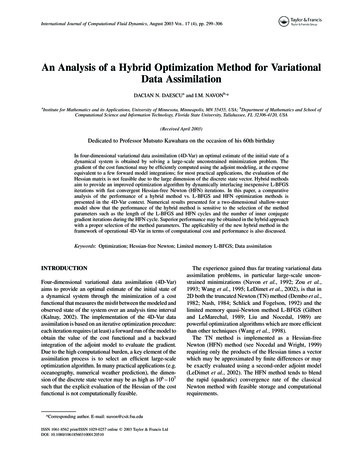
OPTIMIZATION FOR VARIATIONAL DATA ASSIMILATION301The Truncated Newton AlgorithmThe Hybrid MethodIn this method, a search direction is computed by findingan approximate solution to the Newton equationsThe hybrid method aims at dynamically combining thebest features of both systems in the manner of alternatingl steps of L-BFGS with t steps of HFNG k p k ¼ 2g k ;ð2Þwhere p k is a descent direction and Gk is the Hessianmatrix of the cost function G k ¼ 72 f ðx k Þ:The use of an approximate search direction is justifiedby the fact that an exact solution of the Newton equation ata point far from the minimum is computationally wastefulin the framework of a basic descent method. Thus, foreach outer iteration (2) there is an inner iteration loopapplying the conjugate gradient method that computesthis approximate direction, p k , and attempts to satisfy atermination test of the form:kr k k # hk kg k kwhererk ¼ Gkpk þ gkand the sequence {hk} satisfies 0 , hk , 1 for all k.The conjugate gradient inner algorithm is preconditioned by a scaled two-step limited memory BFGS methodin Nash TN method with Powell’s restarting strategy usedto reset the preconditioner periodically. A detaileddescription of the preconditioner may be found in Nash(1985).In the TN method, given a vector v, the Hessian/vectorproduct Gkv required by the inner conjugate gradientalgorithm may be obtained by a finite differenceapproximation,G k v ½gðx k þ hvÞ 2 gðx k Þ h:l*ðL – BFGSÞ ! t*ðHFNðPCGÞÞ ! HðmÞ;repeatwhere H(m) is a limited memory matrix approximating theinverse of the Hessian while m denotes the number ofcorrection pairs stored.In the L-BFGS cycle, H(m) (starting say from the initialunit, or weighted unit matrix) is updated using most recentm pairs. The matrix obtained at the end of L-BFGS cycle isused to precondition the first of the t HFN iterations. In theremaining t 2 1 iterations the limited memory matrixH(m) is updated using information generated by the innerpreconditioned conjugate-gradient (PCG) iteration and itis used to precondition the next HFN iteration. A detaileddescription of the preconditioning process is presentedby Morales and Nocedal (2001). At the end of t HFN steps,the most current H(m) matrix is used as the initial matrixin a new cycle of L-BFGS steps.THE OPTIMIZATION PROBLEMIn this section, we present the variational data assimilationproblem for a two-dimensional shallow-water model.The simplicity of the shallow water equations facilitatesa thorough investigation of various numerical methods(Williamson et al., 1992) while capturing importantcharacteristics present in more comprehensive oceanographic and atmospheric models.The Shallow Water ModelA major issue is how to adequately choose h; in thiswork we usepffiffiffih ¼ e ð1 þ kx k k2 ÞIn a Cartesian coordinate system, the dynamical model isrepresented as a system of nonlinear partial differentialequationswhere e is the machine precision. The inner algorithm isterminated using the quadratic truncation test, whichmonitors a sufficient decrease of the quadratic model›u›u›u›fþ u þ v 2 fv þ¼0›t›x›y›xð3Þ›v›v›v›fþ u þ v þ fu þ¼0›t›x›y›yð4Þ›f ›uf ›v fþþ¼0›t›x›yð5Þqk ¼pTk G k p k 2 þ pTk g ki ð1 2 qi21k Þ qk #cq iwhere i is the counter for the inner iteration and cq is atolerance, satisfying 0 , cq , 1:Ifcq # k7f ðx k Þkthen the truncated-Newton method will convergequadratically (see Dembo et al., 1982; Nash and Sofer,1990; 1996). This fact explains the faster rate ofconvergence and the better quality of results obtainedwith the TN method. For similar results in optimal controlsee LeDimet et al. (2002).where u and v are the components of the horizontalvelocity, f is the geopotential and f the Coriolisparameter. The spatial domain considered is a 6000 km 4400 km channel with a uniform 21 21 spatial grid, suchthat the dimension of the discrete state vector x ¼ ðu; v; fÞis 1083. The initial conditions are specified as inGrammeltvedt (1969) and the model is integrated for10 h using a leap-frog scheme with a time incrementDt ¼ 600 s: The geopotential at t0 ¼ 0 and t ¼ 10 h isdisplayed in Fig. 1.
302D.N. DAESCU AND I.M. NAVONFIGURE 1 The configuration of the geopotential (m2 s22) for the reference run at the initial time t ¼ 0 h and at t ¼ 10 h:4D-Var Data AssimilationThe data assimilation problem is implemented in anidealized framework (twin experiments) by considering atruth and a control experiment with the initial conditionsas control parameters. We assume that the initialconditions described in the previous section representthe true (reference) state xref0 and the model trajectoryx ref(t) obtained during the reference run is used to provideobservations. Next, the initial conditions xref0 are perturbedwith random values chosen from a uniform distribution toobtain a perturbed state xp0 that serves as initial conditionsfor the control run. In Fig. 2, we show the configuration ofthe perturbed geopotential at t0 and after a 10 h run. A costfunctional that measures the least-squares distancebetween the reference run x ref and the control run x inthe assimilation window ½0; 10 h is defined as follows:n T 1Xxðti Þ 2 x ref ðti Þ W i xðti Þ
analysis of the performance of a hybrid method vs. L-BFGS and HFN optimization methods is presented in the 4D-Var context. Numerical results presented for a two-dimensional shallow-water model show that the performance of the hybrid method is sensitive to the selection of the method parameters such as the length of the L-BFGS and HFN cycles and the number of inner conjugate gradient