WIXLIB

Practical Issues in the Analysis of Univariate GARCHModels Eric Zivot†April 18, 2008AbstractThis paper gives a tour through the empirical analysis of univariate GARCHmodels for financial time series with stops along the way to discuss various practical issues associated with model specification, estimation, diagnostic evaluationand forecasting.1IntroductionThere are many very good surveys covering the mathematical and statistical properties of GARCH models. See, for example, [9], [14], [74], [76], [27] and [83]. Thereare also several comprehensive surveys that focus on the forecasting performanceof GARCH models including [78], [77], and [3]. However, there are relatively fewsurveys that focus on the practical econometric issues associated with estimatingGARCH models and forecasting volatility. This paper, which draws heavily from[88], gives a tour through the empirical analysis of univariate GARCH models forfinancial time series with stops along the way to discuss various practical issues.Multivariate GARCH models are discussed in the paper by [80]. The plan of this paper is as follows. Section 2 reviews some stylized facts of asset returns using exampledata on Microsoft and S&P 500 index returns. Section 3 reviews the basic univariateGARCH model. Testing for GARCH effects and estimation of GARCH models arecovered in Sections 4 and 5. Asymmetric and non-Gaussian GARCH models are discussed in Section 6, and long memory GARCH models are briefly discussed in Section7. Section 8 discusses volatility forecasting, and final remarks are given Section 91 .1

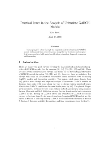
AssetMeanMedMinMaxStd. DevDaily ReturnsMSFT0.0016 0.0000 -0.3012 0.1957 0.0253S&P 500 0.0004 0.0005 -0.2047 0.0909 0.0113Monthly ReturnsMSFT0.0336 0.0336 -0.3861 0.4384 0.1145S&P 500 0.0082 0.0122 -0.2066 0.1250 0.0459Notes: Sample period is 03/14/86 - 06/30/03 giving 1845 4.004 9.922-0.8377 5.186 65.75daily observations.Table 1: Summary Statistics for Daily and Monthly Stock Returns.2Some Stylized Facts of Asset ReturnsLet Pt denote the price of an asset at the end of trading day t. The continuouslycompounded or log return is defined as rt ln(Pt /Pt 1 ). Figure 1 plots the dailylog returns, squared returns, and absolute value of returns of Microsoft stock andthe S&P 500 index over the period March 14, 1986 through June 30, 2003. Thereis no clear discernible pattern of behavior in the log returns, but there is some persistence indicated in the plots of the squared and absolute returns which representthe volatility of returns. In particular, the plots show evidence of volatility clustering - low values of volatility followed by low values and high values of volatilityfollowed by high values. This behavior is confirmed in Figure 2 which shows thesample autocorrelations of the six series. The log returns show no evidence of serialcorrelation, but the squared and absolute returns are positively autocorrelated. Also,the decay rates of the sample autocorrelations of rt2 and rt appear much slower,especially for the S&P 500 index, than the exponential rate of a covariance stationary autoregressive-moving average (ARMA) process suggesting possible long memorybehavior. Monthly returns, defined as the sum of daily returns over the month, areillustrated in Figure 3. The monthly returns display much less volatility clusteringthan the daily returns.Table 1 gives some standard summary statistics along with the Jarque-Bera testfor normality. The latter is computed asÃ!d 3)2T [ 2 (kurtskew ,(1)JB 64d denotes the sample kurtosis. Under[ denotes the sample skewness and kurtwhere skewthe null that the data are iid normal, JB is asymptotically distributed as chi-square The paper was prepared for the Handbook of Financial Time Series, edited by T.G. Andersen,R.A. Davis, J-P Kreiss, and T. Mikosch. Thanks to Saraswata Chaudhuri, Richard Davis, RonSchoenberg and Jiahui Wang for helpful comments and suggestions. Financial support from theGary Waterman Distinguished Scholarship is greatly appreciated.†Department of Economics, Box 353330, University of Washington. ezivot@u.washington.edu.1All of the examples in the paper were constructed using S-PLUS 8.0 and S FinMetrics 2.0. Scriptfiles for replicating the examples may be downloaded from http://faculty.washington.edu/ezivot.2

S & P 500 Returns-0.30-0.200.100.05Microsoft Returns198619901994199820021986199419982002S & P 500 Squared Returns0.000.0000.080.040Microsoft Squared 00.000.30S & P 500 Absolute Returns0.30Microsoft Absolute 2Figure 1: Daily returns, squared returns and absolute returns for Microsoft and theS&P 500 index.with 2 degrees of freedom. The distribution of daily returns is clearly non-normalwith negative skewness and pronounced excess kurtosis. Part of this non-normalityis caused by some large outliers around the October 1987 stock market crash andduring the bursting of the 2000 tech bubble. However, the distribution of the datastill appears highly non-normal even after the removal of these outliers. Monthlyreturns have a distribution that is much closer to the normal than daily returns.3The ARCH and GARCH Model[33] showed that the serial correlation in squared returns, or conditional heteroskedasticity, can be modeled using an autoregressive conditional heteroskedasticity (ARCH)model of the formyt Et 1 [yt ] t ,t2σt(2) zt σ t , a0 a1(3)2t 13 · · · ap2t p ,(4)

S&P 500 Returns0.00.0ACF0.6ACF0.6Microsoft Returns0510Lag1520010Lag15200.00.0ACF0.6S&P 500 Squared ReturnsACF0.6Microsoft Squared Returns50510Lag1520010Lag15200.00.0ACF0.6Microsoft Absolute ReturnsACF0.6Microsoft Absolute Returns50510Lag15200510Lag1520Figure 2: Sample autocorrelations of rt , rt2 and rt for Microsoft and S&P 500 index.where Et 1 [·] represents expectation conditional on information available at time t 1,and zt is a sequence of iid random variables with mean zero and unit variance. In thebasic ARCH model zt is assumed to be iid standard normal. The restrictions a0 0and ai 0 (i 1, . . . , p) are required for σ 2t 0. The representation (2) - (4) isconvenient for deriving properties of the model as well as for specifying the likelihoodfunction for estimation. The equation for σ 2t can be rewritten as an AR(p) processfor 2t222(5)t a0 a1 t 1 · · · ap t p ut ,where ut 2t σ 2t is a martingale difference sequence (MDS) since Et 1 [ut ] 0 andit is assumed that E( 2t ) . If a1 · · · ap 1 then t is covariance stationary,the persistence of 2t and σ 2t is measured by a1 · · · ap and σ̄ 2 var( t ) E( 2t ) a0 /(1 a1 · · · ap ).An important extension of the ARCH model proposed by [12] replaces the AR(p)representation in (4) with an ARMA(p, q) formulationσ 2t a0 pXai 2t ii 1 qXbj σ 2t j ,(6)j 1where the coefficients ai (i 0, · · · , p) and bj (j 1, · · · , q) are all assumed to be4

S&P 500 Returns-0.20-0.30.40.10Microsoft Returns198619901994199820021986199419982002S&P 500 Squared Returns0.020.0050.18Microsoft Squared 0.0ACF0.6S&P 500 Squared ReturnsACF0.6Microsoft Squared Returns19900510Lag15200510Lag1520Figure 3: Monthly Returns, Squared Returns and Sample Autocorrelations ofSquared Returns for Microsoft and the S&P 500.positive to ensure that the conditional variance σ 2t is always positive.2 The model in(6) together with (2)-(3) is known as the generalized ARCH or GARCH(p, q) model.The GARCH(p, q) model can be shown to be equivalent to a particular ARCH( )model. When q 0, the GARCH model reduces to the ARCH model. In order forthe GARCH parameters, bj (j 1, · · · , q), to be identified at least one of the ARCHcoefficients ai (i 0) must be nonzero. Usually a GARCH(1,1) model with onlythree parameters in the conditional variance equation is adequate to obtain a goodmodel fit for financial time series. Indeed, [49] provided compelling evidence that isdifficult to find a volatility model that outperforms the simple GARCH(1,1).Just as an ARCH model can be expressed as an AR model of squared residuals, aGARCH model can be expressed as an ARMA model of squared residuals. Considerthe GARCH(1,1) model(7)σ 2t a0 a1 2t 1 b1 σ 2t 1 .Since Et 1 ( 2t ) σ 2t , (7) can be rewritten as2t a0 (a1 b1 )22t 1 ut b1 ut 1 ,(8)Positive coefficients are sufficient but not necessary conditions for the positivity of conditionalvariance. See [72] and [23] for more general conditions.5

which is an ARMA(1,1) model with ut 2t Et 1 ( 2t ) being the MDS disturbanceterm.Given the ARMA(1,1) representation of the GARCH(1,1) model, many of itsproperties follow easily from those of the corresponding ARMA(1,1) process for 2t .For example, the persistence of σ 2t is captured by a1 b1 and covariance stationarityrequires that a1 b1 1. The covariance stationary GARCH(1,1) model has anARCH( ) representation with ai a1 bi 11 , and the unconditional variance of t isσ̄ 2 a0 /(1 a1 b1 ).For the general GARCH(p, q) model (6), the squared residualst behaveP like anPARMA(max(p, q), q) process. Covariance stationarity requires pi 1 ai qj 1 bi 1and the unconditional variance of t isσ̄ 2 var( t ) 1 3.1³Ppa0i 1 aiConditional Mean Specification Pqj 1 bi .(9)Depending on the frequency of the data and the type of asset, the conditional meanEt 1 [yt ] is typically specified as a constant or possibly a low order autoregressivemoving average (ARMA) process to capture autocorrelation caused by market microstructure effects (e.g., bid-ask bounce) or non-trading effects. If extreme or unusual market events have happened during sample period, then dummy variablesassociated with these events are often added to the conditional mean specification toremove these effects. Therefore, the typical conditional mean specification is of theformrsLXXXφi yt i θj t j β0l xt l t ,(10)Et 1 [yt ] c i 1j 1l 0where xt is a k 1 vector of exogenous explanatory variables.In financial investment, high risk is often expected to lead to high returns. Although modern capital asset pricing theory does not imply such a simple relationship,it does suggest that there are some interactions between expected returns and risk asmeasured by volatility. Engle, Lilien and Robins (1987) proposed to extend the basicGARCH model so that the conditional volatility can generate a risk premium whichis part of the expected returns. This extended GARCH model is often referred toas GARCH-in-the-mean or GARCH-M model. The GARCH-M model extends theconditional mean equation (10) to include the additional regressor g(σ t ), which canbe an arbitrary function of conditional volatility σ t . The most common specificationsare g(σ t ) σ 2t , σ t , or ln(σ 2t ).3.2Explanatory Variables in the Conditional Variance EquationJust as exogenous variables may be added to the conditional mean equation, exogenous explanatory variables may also be added to the conditional variance formula (6)6