WIXLIB

rejection method [20]. We generate a random number, η in [0, 1) when weperform a WOS step, and compare η with p(d), the survival probability at d,the radius of the current sphere in WOS. If η p(d), the random walker isremoved at this WOS step.The estimate for the solution of the LPBE at x0 , the starting point of theMarkov chain, is given by SN :Ns1 XSN ψ0 (Xni ).N i 1(9)Here, N is the total number of random walkers, Ns is the number of survivedand-absorbed random walkers, and Xni is the final position of the walker onthe boundary when it is absorbed after ni WOS steps. In this method, like theWOS method, errors are due to both statistical sampling and the ε-absorptionlayer which captures random walkers near the boundary to terminate theconstruction of the Markov chain. However, the error from the ε-absorptionlayer can always be made smaller than the statistical error [15,16]. On thesame random walk, estimating the solution for different values of ε allowsone to approximate δ(ε), the error as a function of ε [14]. On the one hand,by adjusting ε, we can make the error from the absorption layer less thanthe statistical error. This means that if we increase the number of randomwalkers in order to decrease the statistical error, consequently we must reduceε, and thus increases the running time, as O(log ε) [14]. On the other hand, ifone fixes the desired accuracy, then the bias and the statistical error can beadjusted to have the same order. This means that it is theoretically possibleto choose the number of random walkers, N , beforehand.In the following, we compare our simulation results with the known analyticresults for four problems [2], which were used as test problems for the discreterandom walk method [11]. The problems are to find the solution of the firstboundary-value problem for the LPBE (4),(5) in four different domains: a)outside of a charged sphere with the radius of the unit Debye length; b) awayfrom the infinitely long cylinder with the radius of the unit Debye length;c) away from the infinite flat surface; d) between two parallel flat plates 3Debye lengths apart from each other. In all cases, the results are given asthose normalized by the constant boundary condition, ψ0 , which is assumedto be sufficiently small for the LPBE to be valid. The number of random walksused for computing the solution at a point is 105 , and the absorption layerthickness is ε 10 4 . The analytic results [11] are shown with solid lines inFig. 2 and our simulation results with circles. For all four cases, our simulationresults show excellent agreement.Our method has several features. First, it is easier to implement and is expected to be faster than the other discretized methods, such as the discrete6

0.40.40.30.30.20.20.10.1000.511.5 1r (in units of κ )22.50300.511.522.5 1r (in units of κ 0.40.60.30.20.50.100123 1r (in units of κ )40.4 1.55 1 0.500.5 1r (in units of κ )11.5Fig. 2. The solid lines are the analytic solutions and the circles are the simulationresults with 105 random walks and the width of absorption layer, ε 10 4 . Here,κ is the inverse Debye length. (a) Electric potential away from the surface of acharged sphere in an electrolyte; Here, r is the distance from the surface of thesphere with unit radius. (b) Electric potential away from an infinitely long chargedcylinder in an electrolyte; Here, r is the distance from the surface of the cylinderwith unit radius. (c) Electric potential away from an charged infinite flat plate inan electrolyte; Here, r is the distance from the plate. (d) Electric potential in anelectrolyte between two infinite charged parallel flat plates; Here, r is the distancefrom the mid-point between two plates.random walk method [11], the finite difference method [21] and the boundaryelement method [22], especially with complicated geometries. For the solutionat a point, it takes only a few seconds to compute it with 105 random walkersand ε 10 4 on a 550 Mhz PC. However, it is hard to compare this methodto other methods because they compute solutions at all grid points. We cansafely say that continuous Monte Carlo methods are more efficient when thesolution is required only at relatively small number of points. Secondly, the accuracy and the running time of our method depends primarily on the numberof statistical samples. Naturally, these samples can be simulated in parallel.Thirdly, it is certain that our method is faster than the old WOS method [1],because while some of our random walkers are removed during the simulation,in the old method all trajectories must be completed and contribute to thesolution according to the calculated weights. Also, in the unbounded domaincases, like the three examples, not the parallel plates, it is necessary to use7

Table 1The computational cost comparison of our algorithm with the old modified WOSin the case of parallel plates at the mid-point; the variances are obtained from 100independent runs, the number of random walks per run is 105 and the width ofabsorption layer, ε 10 4 .methodCPU time per runvariancecomputational cost(secs)(10 7 )(10 6 )old method13.474.636.24our method2.9719.85.88a certain cut-off in the old modified WOS [1] to kill random walkers, whichwill bias the results. As an example, in Table 1, for the case of the parallelplates, we compare our method with the old modified WOS method [1]. Weuse a conventional comparison criterion for the Monte Carlo methods, thecomputational cost (or time consumption) [23,20]: t σ 2 [ξ], where t is theCPU time needed to calculate a single sample of the estimate, and σ 2 [ξ] is thevariance of the estimate. The less laborious the algorithm, the more efficientit is. The computational results in Table 1 show that the computational costof our algorithm is less than that of the old modified WOS method. Finally,our method is easy to extend to solve the LPBE with source terms.3Feynman-Kac “Walks on Spheres”In this section 2 , we present a new modified WOS method for solving theDirichlet problem for the LPBE based on the Feynman-Kac formula [3]. Inaddition, we show that this method is mathematically equivalent to our previous modified WOS method [3]. According to the Feynman-Kac formula, thesolution to the first boundary value problem for the LPBE at the point x0is [12,24]τ ΩZκ2 dτ }] ,u(x0 ) E[ψ0 (X(τ Ω )) exp{ (10)0where X(τ ) is a Brownian motion trajectory, τ Ω inf{τ : X(τ ) Ω} is thefirst-passage time of this trajectory, and X(τ Ω ) is the first-passage point onthe boundary. If we use a series of WOS steps to construct a Brownian path2This section is based on: C.-O. Hwang, M. Mascagni and J.A. Given, “A FeynmanKac Formula Implementation for the Linearized Poisson-Boltzmann Equation,”Math. Comput. Simulation. submitted, (2002)8

10.90.80.7P(dκ)0.6Feynman KacElepov Mikhailov0.50.40.30.20.10012345dκ678910Fig. 3. The survival probability density function; the dashed line shows the survivalprobability from the Feynman-Kac solution representation [12,24] with only the firstmoment of the first passage time distribution function; the solid line is the survivalprobability from the Elepov-Mikhailov solution representation [1]; d is the distanceof a random walker from the starting position, and κ is the inverse Debye length.with only the first moment of the first passage time distribution function (seee.g. [17]), the corresponding survival probability (Feynman-Kac in Fig. 3) isexp( κ2 r2 /6) ,(11)where r is the radius of each WOS (see Fig. 3 to compare with the previous Elepov-Mikhailov removal probability). The survival probability from theFeynman-Kac formula using the mean of the first passage time can be usedonly when r is small enough (less than 1 in units of κ 1 ). If r is large, theentire first passage time distribution function (see Fig. 4)P (t0 ) 1 2 X( 1)n exp( n2 π 2 t0 ),(12)n 1should be used, not just the mean. Here, t0 Dτ /r2 where D is the diffusionconstant (in the LPBE, D 1), τ is the first passage time, and r is the radiusof the WOS step. To use this distribution function, we tabulate it.At every WOS step, after sampling t0 , the corresponding survival probabilityis obtained. The survival probability is compared with a random number in[0, 1) and if the random number is greater than the survival probability, therandom walker is removed at this WOS step: the acceptance-rejection method.The estimated solution of the LPBE at x0 , where the random walkers start,9

. 4. The first passage time distribution function for spheres with respect to thenormalized time t0 : here, t0 Dτ /r2 and D 1 is the diffusion constant, τ is thefirst passage time, and r is the radius of the sphere.isNs1 XE(x0 ) ψ0 (Xni ).N i 1(13)Here, N is the total number of random walkers, Ns is the number of survivedand-absorbed trajectories, and Xni is the nearest point on the boundary towhere the walker hits the ε-absorption layer for the first time, ni is the randomnumber of WOS steps in the ith trajectory. Mathematically, this new survivalprobability density function derived with the entire first-passage time distribution function, is equivalent to the previous survival probability density for thefollowing reason: the expected value of the exponential weight factor at everyWOS step in our new Feynman-Kac formula implementation with respect tothe entire first-passage time distribution function is equivalent to the previous Elepov-Mikhailov survival distribution function. To show it, we computethe average of the exponential weight factor, exp( t0 κ2 r2 ) (for D 1), withrespect to the probability density of t0 :Z 0 2 20exp( t κ r )dP (t ) 20 XZ n2 2exp[ (n2 π 2 κ2 r2 )t0 ]dt0( 1) ( n π )n 10 Xn( 1)2 22 2n 1 1 κ r /(n π )κr .sinh(κr) 210(14)

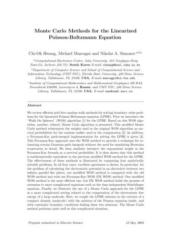
0.40.40.30.30.20.20.10.10000.511.5 1r (in units of κ )22.5300.5(a)11.522.5 1r (in units of κ .50.70.40.60.30.20.50.100123 1r (in units of κ )40.4 1.55(c) 1.0 0.50.00.5 1r (in units of κ )1.01.5(d)Fig. 5. The solid lines are the analytic solutions and the circles are the simulationresults with 106 random walks and the absorption layer ε 10 4 ; here, κ is theinverse Debye length. (a) Electric potential away from the surface of a charged spherein the electrolyte; here, r is the distance from the surface of the sphere with unitradius. (b) Electric potential away from the infinitely long charged cylinder in theelectrolyte; here, r is the distance from the surface of the cylinder with unit radius.(c) Electric potential away from the charged infinite flat plate in the electrolyte; here,r is the distance from the plate. (d) Electric potential in the electrolyte betweentwo infinite charged parallel flat plates; here, r is the distance from the mid-pointof the plates.This is the same as the survival probability in our previous modified WOSmethod [2].The efficiency of this method is illustrated by computing the same four analytically solvable problems that were considered in the previous section. Wecompare our simulation results with known analytic expressions [11]. In allcases, the results are normalized by the boundary condition, ψ0 . The number of random walks used for finding the solution at a point is 106 , and theabsorption layer thickness is ε 10 4 . In Fig. 5 the analytic results [11]are shown with the solid lines and our computed results are represented bycircles. For all four cases, our simulation results show excellent agreement.Also, in the case of the electric potential in an electrolyte between two infinite charged parallel flat plates, we compare the FK WOS algorithm with our11

previous one. The FK WOS method is slower because of the computationaltime spent on the interpolation routine when sampling t0 . In Table 2, runningtimes are given for the case when the piecewise linear interpolation is usedto sample t0 . While this method is somewhat slower than our previous one,it holds the promise of extension to more complicated equations such as thetime-independent Schrödinger or Bloch equations.4Error and Running TimeIn this section 3 , we investigate the relationship between the running timeand the thickness of the ε-absorption layer, and the error associated withthe this layer in both the modified WOS and FK WOS algorithms, and givenumerical illustrations. There are two error sources in these methods; the errorassociated with the number of trajectories (sampling error), and the errorassociated with the ε-absorption layer. We can reduce the statistical samplingerror by increasing the number of trajectories. The error associated with theε-absorption layer can be reduced by reducing ε, the layer thickness. However,increasing the number of trajectories will increase the running time linearly,while reducing ε will increase running time as O( log ε ) [14]. In the case of FKWOS in Fig. 6 (a), we see the usual logarithmic relationship between runningtime and the thickness of the ε-absorption layer. The reason for this is thatthe running time increases proportionally to the number of WOS steps, ni ,which is itself O( log ε ) [14]. This relation holds even though some of thetrajectories are terminated during the WOS steps.The error from the ε-absorption layer can be investigated empirically if we haveenough trajectories so that the statistical sampling error is much smaller than3This section is based on: C.-O. Hwang, M. Mascagni and J.A. Given, “A FeynmanKac Formula Implementation for the Linearized Poisson-Boltzmann Equation”,Math. Comput. Simulation submitted, (2002)Table 2Running time comparison of the Feynman-Kac WOS algorithm with our previousmodified WOS in the case of computing the potential in the middle between parallelplates; the number of random walks per run is 106 and the width of absorption layer,ε 10 4 . Both computations were performed on a 550 MHz Pentium workstation.methodCPU time per run (secs)previous method48.9new method64.512

200.02absolute errorrunning time (secs)0.015150.01100.005running time datalogarithmic regression5 710 610 5 4 3101010 1ε absorption layer (in units of κ ) 210100 1simulation errorlinear regression00.01 0.02 0.03 0.04 0.05 0.06 0.07 0.08 0.09 1ε absorption layer (in units of κ )0.1Fig. 6. Running time versus the thickness of the ε-absorption layer and error arisingfrom the ε-absorption layer in Feynman-Kac WOS. (a) Running time versus thethickness of the ε-absorption layer with 106 Brownian trajectories in the case ofcomputing the potential in the middle between the parallel plates. This shows theusual relation for WOS: running time (proportional to number of WOS steps foreach Brownian trajectory) is O( log ε ). (b) Error arising from the ε-absorption layerwith 108 Brownian trajectories in the case of parallel plates in units of κ 1 . Theerror is linear in ε.the bias from using the ε-absorption layer [26]. Fig. 6 (b) shows the empiricalresults with 108 Brownian trajectories: the ε-layer error grows linearly in ε forsmall ε just as in the case of the Dirichlet problem for the Laplace or Poissonequations [26]. The reason is that for small ε the probability of terminating aBrownian trajectory is linear in ε.5Biochemical ApplicationIn this section 4 , we consider the problem of calculating the internal energyof a molecule. To be more exact, we will calculate the electrostatic energy –the internal energy for non-bonded electrostatic interactions between atomsconstituting a large molecule.In biochemical applications, one of the possible and widely used electrostaticmodels is a continuum model. For a given charge distribution ρ(x), the electrostatic potential is determined as a solution to Poisson’s equation ² ψ(x) ρ(x) , x R3 ,(15)where ² is a position-dependent permittivity. In bio-molecular applications,4This section is based on: M. Mascagni and N.A. Simonov, “Monte Carlo Methodfor Calculating the Electrostatic Energy of a Molecule”, presented at ICCS-2003,St.Petersburg, Russia, June 2-4, 2003. To be published in LNCS by Springer-Verlag.13

the geometry of a problem is taken into account by thinking of a molecule asa cavity with point charges and constant ² inside. The exterior is modelled asa dielectric medium with different permittivity and some charge distribution.We assume that the molecule in question can be described as a compact setΩ R3 constructed of a large number of intersecting balls (atoms). Everyspherical atom has its electrical charge, qm , which is positioned at its center,xm , and rm is the radius of this atom. Hence, the electrostatic potential, ψ(x),satisfies Poisson’s equation (15) inside Ω for the particular charge densityρ(x) MXqm δ(x xm ). Here, the dielectric permittivity, ² ²i , is constant.m 1The potential can be represented as the sum of two functions:ψ(x) ψ (0) (x) g(x) ,(16)MXqm1. From (16) and (15) it follows that ψ (0) (x) 4π² x x imm 10 in Ω, and the boundary values of ψ (0) are equal to ψ(x) g(x). If the moleculeis surrounded by some dielectric (e.g. water), the classical approach is to treatthis surrounding medium as continuous with some constant permittivity, ²e .The distribution of dissolved ions determines the charge density outside Ω,which leads to the non-linear Poisson-Boltzmann equation (1) in the exteriordomain G1 R3 \ G. Linearizing it for small potential values, we come to theLPBE (2), where k is determined by (3) with the permittivity ²e .where g(x) Equations (15) and (2) must be coupled by continuity conditions on the boundary of the molecule:ψi (y) ψe (y) , ²i ψi ψe ²e, y G . n(y) n(y)(17)Here, for convenience, we denote ψi as the solution to (15) in the interior ofΩ, and ψe as the solution of (2) in the exterior of the molecule. We assumealso that ψe (x) 0 as x goes to infinity.In the linear case the electrostatic free energy of the molecule is given by [27]:E M1 Xψm qm ,2 m 1(18)where ψm is the non-singular part of the electrostatic potential at the centerof the m-th atom. This means that in the calculation of E we exclude theinfinite self-energy of the point charges, and take ψm ψ (0) (xm ).To find the energy, E, we construct a Monte Carlo algorithm based on the14

properties of Brownian motion. Denote by ξ[E] a Monte Carlo estimate forE. We represent it as a weighted sum of estimators for point values of thepotential:ξ[E] M1 Xξ[ψm ] qm .2 m 1Construction of every ξ[ψm ] ξ[ψ (0) ](xm ) is based on the simulation of a(0)WOS Markov chain {x(j)m , j 0, 1, . . . , Nm } with initial point xm xm , m 1, . . . , M and random length Nm . The geometry of the domain Ω makes itm)possible to simulate exit points x(N Ω exactly. So we havemhi(Nm )m)ψm E ψ(x(N) g(xm) .m(19)To estimate the unknown boundary values, we make use of the boundaryconditions (17). We implement a finite-dif

Monte Carlo Methods for the Linearized Poisson-Boltzmann Equation Chi-Ok Hwang, Michael Mascagni and Nikolai A. Simonova;b;c aComputational Electronics Center, Inha University, 253 Yonghyun-Dong Nam-Gu, Incheon 402-751, South Korea E-mail: chwang@hsel.inha.ac.kr bDepartment of Computer Science and School of Computational Science and Information Technology (CSIT FSU), Florida State University .