Transcription
Algebraic FoundationsforTopological Data AnalysisDRAFT 15 January 2022Hal SchenckD EPARTMENT OF M ATHEMATICS AND S TATISTICS , AUBURN U NIVERSITYEmail address: hks0015@auburn.edu
c 2021 Hal Schenck
PrefaceThis book is a mirror of applied topology and data analysis: it covers a wide rangeof topics, at levels of sophistication varying from the elementary (matrix algebra)to the esoteric (Grothendieck spectral sequence). My hope is that there is something for everyone, from undergraduates immersed in a first linear algebra class tosophisticates investigating higher dimensional analogs of the barcode. Readers areencouraged to barhop; the goal is to give an intuitive and hands on introduction tothe topics, rather than a punctiliously precise presentation.The notes grew out of a class taught to statistics graduate students at AuburnUniversity during the COVID summer of 2020. The book reflects that: it is writtenfor a mathematically engaged audience interested in understanding the theoreticalunderpinnings of topological data analysis. Because the field draws practitionerswith a broad range of experience, the book assumes little background at the outset.However, the advanced topics in the latter part of the book require a willingness totackle technically difficult material.To treat the algebraic foundations of topological data analysis, we need to introduce a fair number of concepts and techniques, so to keep from bogging down,proofs are sometimes sketched or omitted. There are many excellent texts on upperlevel algebra and topology where additional details can be found, for example:Algebra ReferencesAluffi [2]Artin [3]Eisenbud [70]Hungerford [93]Lang [102]Rotman [132]Topology ReferencesFulton [76]Greenberg–Harper [83]Hatcher [91]Munkres [119]Spanier [137]Weibel [149]iii
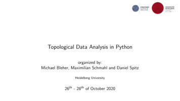
ivPrefaceTechniques from linear algebra have been essential tools in data analysis from thebirth of the field, and so the book kicks off with the basics: Least Squares Approximation Covariance Matrix and Spread of Data Singular Value DecompositionTools from topology have recently made an impact on data analysis. This textprovides the background to understand developments such as persistent homology.Suppose we are given point cloud data, that is, a set of points X:If X was sampled from some object Y , we’d like to use X to infer propertiesof Y . Persistent Homology applies tools of algebraic topology to do this. We startby using X as a seed from which to grow a family of spaces[X N (p), where N (p) denotes an ball around p.p XAs X X 0 if 0 , we have a family of topological spaces and inclusion maps.As Weinberger notes in [150], persistent homology is a type of Morse theory:there are a finite number of values of where the topology of X changes. Notice that when 0, X is a giant blob; so is typically restricted to a range[0, x]. Topological features which “survive” to the parameter value x are said to bepersistent; in the example above the circle S 1 is a persistent feature.The first three chapters of the book are an algebra-topology boot camp. Chapter 1 provides a brisk review of the tools from linear algebra most relevant forapplications, such as webpage ranking. Chapters 2 and 3 cover the results we needfrom upper level classes in (respectively) algebra and topology. Applied topologyappears in §3.4, which ties together sheaves, the heat equation, and social media.Some readers may want to skip the first three chapters, and jump in at Chapter 4.
PrefacevThe main techniques appear in Chapter 4, which defines simplicial complexes,simplicial homology, and the Čech & Rips complexes. These concepts are illustrated with a description of the work of de Silva–Ghrist using the Rips complex toanalyze sensor networks. Chapter 5 further develops the algebraic topology toolkit,introducing several cohomology theories and highlighting the work of Jiang–Lim–Yao–Ye in applying Hodge theory to voter ranking (the Netflix problem).We return to algebra in Chapter 6, which is devoted to modules over a principal ideal domain–the structure theorem for modules over a principal ideal domain plays a central role in persistent homology. Chapters 7 and 8 cover, respectively, persistent and multiparameter persistent homology. Chapter 9 is the piècede résistance (or perhaps the coup de grâce)–a quick and dirty guide to derivedfunctors and spectral sequences. Appendix A illustrates several of the softwarepackages which can be used to perform computations.There are a number of texts which tackle data analysis from the perspectiveof pure mathematics. Elementary Applied Topology [79] by Rob Ghrist is closestin spirit to these notes; it has a more topological flavor (and wonderfully illuminating illustrations!). Other texts with a similar slant include Topological DataAnalysis with Applications [30] by Carlsson–Vejdemo-Johanssen, ComputationalTopology for Data Analysis [60] by Dey–Wang, and Computational Topology [67]by Edelsbrunner–Harer. At the other end of the spectrum, Persistence theory:from quiver representations to data analysis [124] by Steve Oudot is intended formore advanced readers; the books of Polterovich–Rosen–Samvelyan–Zhang [126],Rabadan–Blumberg [127] and Robinson [131] focus on applications. Statisticalmethods are not treated here; they merit a separate volume.Many folks deserve acknowledgement for their contributions to these notes,starting with my collaborators in the area: Heather Harrington, Nina Otter, andUlrike Tillmann. A precursor to the summer TDA class was a minicourse I taughtat CIMAT, organized by Abraham Martı́n del Campo, Antonio Rieser, and CarlosVargas Obieta. The summer TDA class was itself made possible by the RosemaryKopel Brown endowment, and writing by NSF grant 2048906. Thanks to HannahAlpert, Ulrich Bauer, Michael Catanzaro, David Cox, Ketai Chen, Carl de Boor,Vin de Silva, Robert Dixon, Jordan Eckert, Ziqin Feng, Oliver Gäfvert, Rob Ghrist,Sean Grate, Anil Hirani, Yang Hui He, Michael Lesnick, Lek-Heng Lim, DmitriyMorozov, Steve Oudot, Alex Suciu, and Matthew Wright for useful feedback.Data science is a moving target: one of today’s cutting edge tools may be relegated to the ash bin of history tomorrow. For this reason the text aims to highlightmathematically important concepts which have proven or potential utility in applied topology and data analysis. But mathematics is a human endeavor, so it iswise to remember Seneca: “Omnia humana brevia et caduca sunt.”Hal Schenck
ContentsPrefaceiiiChapter 1.Linear Algebra Tools for Data Analysis1§1.1.Linear Equations, Gaussian Elimination, Matrix Algebra1§1.2.Vector Spaces, Linear Transformations, Basis and Change of Basis5§1.3.Diagonalization, Webpage Ranking, Data and Covariance8§1.4.Orthogonality, Least Squares Fitting, Singular Value Decomposition 14Chapter 2.Basics of Algebra: Groups, Rings, Modules21§2.1.Groups, Rings and Homomorphisms21§2.2.Modules and Operations on Modules24§2.3.Localization of Rings and Modules31§2.4.Noetherian rings, Hilbert basis theorem, Varieties33Chapter 3.Basics of Topology: Spaces and Sheaves37§3.1.Topological Spaces38§3.2.Vector Bundles42§3.3.Sheaf Theory44§3.4.From Graphs to Social Media to Sheaves48Chapter 4.Homology I: Simplicial Complexes to Sensor Networks55§4.1.Simplicial Complexes, Nerve of a Cover56§4.2.Simplicial and Singular Homology58§4.3.Snake Lemma and Long Exact Sequence in Homology62§4.4.Mayer–Vietoris, Rips and Čech complex, Sensor Networks65vii
viiiContentsChapter 5.Homology II: Cohomology to Ranking Problems73§5.1.Cohomology: Simplicial, Čech, de Rham theories74§5.2.Ranking, the Netflix Problem, and Hodge Theory80§5.3.CW Complexes and Cellular Homology82§5.4.Poincaré and Alexander Duality: Sensor Networks Revisited85Chapter 6.Persistent Algebra: Modules over a PID95§6.1.Principal Ideal Domains and Euclidean Domains96§6.2.Rational Canonical Form of a Matrix98§6.3.Linear Transformations, K[t]-Modules, Jordan Form99§6.4.Structure of Abelian Groups and Persistent HomologyChapter 7.Persistent Homology100105§7.1.Barcodes, Persistence Diagrams, Bottleneck Distance106§7.2.Morse Theory114§7.3.The Stability Theorem117§7.4.Interleaving and Categories121Chapter 8.Multiparameter Persistent Homology131§8.1.Definition and Examples132§8.2.Graded algebra, Hilbert function, series, polynomial135§8.3.Associated Primes and§8.4.Filtrations and ExtChapter 9.Zn -gradedmodules140146Derived Functors and Spectral Sequences151§9.1.Injective and Projective Objects, Resolutions152§9.2.Derived Functors153§9.3.Spectral Sequences159§9.4.Pas de Deux: Spectral Sequences and Derived Functors165Appendix A.Examples of Software Packages173§A.1.Covariance and spread of data via R173§A.2.Persistent homology via scikit-tda175§A.3.Computational algebra via Macaulay2179§A.4.Multiparameter persistence via RIVET181Bibliography187
Chapter 1Linear Algebra Tools forData AnalysisWe begin with a short and intense review of linear algebra. There are a numberof reasons for this approach; first and foremost is that linear algebra is the computational engine that drives most of mathematics, from numerical analysis (finiteelement method) to algebraic geometry (Hodge decomposition) to statistics (covariance matrix and the shape of data). A second reason is that practitioners ofdata science come from a wide variety of backgrounds–a statistician may not haveseen eigenvalues since their undergraduate days. The goal of this chapter is todevelop basic dexterity dealing with Linear Equations, Gaussian Elimination, Matrix Algebra. Vector Spaces, Linear Transformations, Basis and Change of Basis. Diagonalization, Webpage Ranking, Data and Covariance. Orthogonality, Least Squares Data Fitting, Singular Value Decomposition.There are entire books written on linear algebra, so our focus will be on examplesand computation, with proofs either sketched or left as exercises.1.1. Linear Equations, Gaussian Elimination, Matrix AlgebraIn this section, our goal is to figure out how to set up a system of equations to studythe following question:Example 1.1.1. Suppose each year in Smallville that 30% of nonsmokers begin tosmoke, while 20% of smokers quit. If there are 8000 smokers and 2000 nonsmokers at time t 0, after 100 years, what are the numbers? After n years? Is there anequilibrium state at which the numbers stabilize?1
21. Linear Algebra Tools for Data AnalysisThe field of linear algebra is devoted to analyzing questions of this type. We nowembark on a quick review of the basics. For example, consider the system of linearequationsx 2y 22x 3y 6Gaussian elimination provides a systematic way to manipulate the equations toreduce to fewer equations in fewer variables. A linear equation (no variable appearsto a power greater than one) in one variable is of the form x constant, so is trivial.For the system above, we can eliminate the variable x by multiplying the first rowby 2 (note that this does not change the solutions to the system), and adding it tothe second row, yielding the new equation 7y 2. Hence y 27 , and substitutingthis for y in either of the two original equations, we solve for x, finding that x 187 .Gaussian elimination is a formalization of this simple example: given a system oflinear equationsa11 x1 a12 x2 · · · a1n xn b1a21 x1 a22 x2 · · · a2n xn b2. . .(a) swap order of equations so a11 6 0.(b) multiply the first row by1a11 ,so the coefficient of x1 in the first row is 1.(c) subtract ai1 times the first row from row i, for all i 2.At the end of this process, only the first row has an equation with nonzero x1coefficient. Hence, we have reduced to solving a system of fewer equations infewer unknowns. Iterate the process. It is important that the operations above donot change the solutions to the system of equations; they are known as elementaryrow operations: formally, these operations are(a) Interchange two rows.(b) Multiply a row by a nonzero constant.(c) Add a multiple of one row to another row.Exercise 1.1.2. Solve the systemx y z 32x y 73x 2z 5You should end up with z 57 , now backsolve. It is worth thinking about thegeometry of the solution set. Each of the three equations defines a plane in R3 .What are the possible solutions to the system? If two distinct planes are parallel,we have equations ax by cz d and ax by cz e, with d 6 e, then thereare no solutions, since no point can lie on both planes. On the other hand, the threeplanes could meet in a single point–this occurs for the system x y z 0, for
1.1. Linear Equations, Gaussian Elimination, Matrix Algebra3which the origin (0, 0, 0) is the only solution. Other geometric possibilities for theset of common solutions are a line or plane; describe the algebra that correspondsto the last two possibilities. There is a simple shorthand for writing a system of linear equations as above usingmatrix notation. To do so, we need to define matrix multiplication.Definition 1.1.3. A matrix is a m n array of elements, where m is the numberof rows and n is the number of columns.Vectors are defined formally in §1.2; informally we think of a real vector v asan n 1 or 1 n matrix with entries in R, and visualize it as a directed arrow withtail at the origin (0, . . . , 0) and head at the point of Rn corresponding to v.Definition 1.1.4. The dot product of vectors v [v1 , . . . , vn ] and w [w1 , . . . , wn ]isnX v·w vi wi , and the length of v is v v · v.i 1By the law of cosines, v, w are orthogonal iff v · w 0, which you’ll prove inExercise 1.4.1. An m n matrix A and p q matrix B can be multiplied whenn p. If (AB)ij denotes the (i, j) entry in the product matrix, then(AB)ij rowi (A) · colj (B).This definition may seem opaque. It is set up exactly so that when the matrix Brepresents a transition from State1 to State2 and the matrix A represents a transitionfrom State2 to State3 , then the matrix AB represents the composite transition fromState1 to State3 . This makes clear the reason that the number of columns of A mustbe equal to the number of rows of B to compose the operations: the target of themap B is the source of the map A.Exercise 1.1.5. 2 31 71 3 ·55263748 37 46 55 Fill in the remainder of the entries. 64 Definition 1.1.6. The transpose AT of a matrix A is defined via (AT )ij Aji .A is symmetric if AT A, and diagonal if Aij 6 0 i j. If A and B arediagonal n n matrices, thenAB BA and (AB)ii aii · biiThe n n identiy matrix In is a diagonal matrix with 1’s on the diagonal; if A isan n m matrix, thenIn · A A A · Im .An n n matrix A is invertible if there is an n n matrix B such that BA AB In . We write A 1 for the matrix B; the matrix A 1 is the inverse of A.
41. Linear Algebra Tools for Data AnalysisExercise 1.1.7. Find a pair of 2 2 matrices (A, B) such that AB 6 BA. Showthat (AB)T B T AT , and use this to prove that the matrix AT A is symmetric. In matrix notation a system of n linear equations in m unknowns is written asA · x b, where A is an n m matrix and x [x1 , . . . , xm ]T .We close this section by returning to our vignette.Example 1.1.8. To start the analysis of smoking in Smallville, we write out thematrix equation representing the change during the first year, from t 0 to t 1.Let [n(t), s(t)]T be the vector representing the number of nonsmokers and smokers(respectively) at time t. Since 70% of nonsmokers continue as nonsmokers, and20% of smokers quit, we have n(1) .7n(0) .2s(0). At the same time, 30%of nonsmokers begin smoking, while 80% of smokers continue smoking, hences(1) .3n(0) .8s(0). We encode this compactly as the matrix equation: n(1)s(1) .7.3.2.8 n(0)·s(0)Now note that to compute the smoking status at t 2, we have n(2)s(2) .7.3.2.8 n(1).7· s(1).3.2.8 .7·.3.2.8 n(0)·s(0)And so on, ad infinitum. Hence, to understand the behavior of the system for t verylarge (written t 0), we need to compute limt .7.3.2.8 t n(0)·s(0)Matrix multiplication is computationally expensive, so we’d like to find a trickto save ourselves time, energy, and effort. The solution is the following, which fornow will be a Deus ex Machina (but lovely nonetheless!) Let A denote the 2 2matrix above (multiply by 10 for simplicity). Then 3/51/5 2/51/5 7·328 1· 123 50010 Write this equation as BAB 1 D, with D denoting the diagonal matrix onthe right hand side of the equation. An easy check shows BB 1 is the identitymatrix I2 . Hence(BAB 1 )n (BAB 1 )(BAB 1 )(BAB 1 ) · · · BAB 1 BAn B 1 Dn ,
1.2. Vector Spaces, Linear Transformations, Basis and Change of Basis5which follows from collapsing the consecutive B 1 B terms in the expression. SoBAn B 1 Dn , and therefore An B 1 Dn B.As we saw earlier, multiplying a diagonal matrix with itself costs nothing, so wehave reduced a seemingly costly computation to almost nothing; how do we find themystery matrix B? The next two sections of this chapter are devoted to answeringthis question.1.2. Vector Spaces, Linear Transformations, Basis and Change ofBasisIn this section, we lay out the underpinnings of linear algebra, beginning with thedefinition of a vector space over a field K. A field is a type of ring, and is definedin detail in the next chapter. For our purposes, the field K will typically be one of{Q, R, C, Z/p}, where p is a prime number.Definition 1.2.1. (Informal) A vector space V is a collection of objects (vectors),endowed with two operations: vectors can be added to produce another vector, ormultiplied by an element of the field. Hence the set of vectors V is closed underthe operations. The formal definition of a vector space appears in Definition 2.2.1.Example 1.2.2. Examples of vector spaces.(a) V Kn , with [a1 , . . . , an ] [b1 , . . . , bn ] [a1 b1 , . . . , an bn ] andc[a1 , . . . , an ] [ca1 , . . . , can ].(b) The set of polynomials of degree at most n 1, with coefficients in K.Show this has the same structure as part (a).(c) The set of continuous functions on the unit interval.If we think of vectors as arrows, then we can visualize vector addition asputting the tail of one vector at the head of another: draw a picture to convinceyourself that[1, 2] [2, 4] [3, 6].1.2.1. Basis of a Vector Space.Definition 1.2.3. For a vector space V , a set of vectors {v1 , . . . , vk } V is linearly independent (or simply independent) ifkXai vi 0 all the ai 0.i 1 a spanning set for V (or simply spans V ) if for any v V there existai K such thatkXai vi v.i 1
61. Linear Algebra Tools for Data AnalysisExample 1.2.4. The set {[1, 0], [0, 1], [2, 3]} is dependent, since 2·[1, 0] 3·[0, 1] 1 · [2, 3] [0, 0]. It is a spanning set, since an arbitrary vector [a, b] a · [1, 0] b · [0, 1]. On the other hand, for V K3 , the set of vectors {[1, 0, 0], [0, 1, 0]} isindependent, but does not span.Definition 1.2.5. A subsetS {v1 , . . . , vk } Vis a basis for V if it spans and is independent. If S is finite, we define the dimensionof V to be the cardinality of S.A basis is loosely analogous to a set of letters for a language where the wordsare vectors. The spanning condition says we have enough letters to write everyword, while the independent condition says the representation of a word in termsof the set of letters is unique. The vector spaces we encounter in this book will befinite dimensional. A cautionary word: there are subtle points which arise whendealing with infinite dimensional vector spaces.Exercise 1.2.6. Show that the dimension of a vector space is well defined.1.2.2. Linear Transformations. One of the most important constructions in mathematics is that of a mapping between objects. Typically, one wants the objects tobe of the same type, and for the map to preserve their structure. In the case ofvector spaces, the right concept is that of a linear transformation:Definition 1.2.7. Let V and W be vector spaces. A map T : V W is a lineartransformation ifT (cv1 v2 ) cT (v1 ) T (v2 ),for all vi V , c K. Put more tersely, sums split up, and scalars pull out.While a linear transformation may seem like an abstract concept, the notion ofbasis will let us represent a linear transformation via matrix multiplication. On theother hand, our vignette about smokers in Smallville in the previous section showsthat not all representations are equal. This brings us to change of basis.Example 1.2.8. The sets B1 {[1, 0], [1, 1]} and B2 {[1, 1], [1, 1]} are easilychecked to be bases for K2 . Write vBi for the representation of a vector v in termsof the basis Bi . For example[0, 1]B1 0 · [1, 0] 1 · [1, 1] 1 · [1, 1] 0 · [1, 1] [1, 0]B2The algorithm to write a vector b in terms of a basis B {v1 , . . . , vn } is asfollows: construct a matrix A whose columns are the vectors vi , then use Gaussianelimination to solve the system Ax b.Exercise 1.2.9. Write the vector [2, 1] in terms of the bases B1 and B2 above.
1.2. Vector Spaces, Linear Transformations, Basis and Change of Basis7To represent a linear transformation T : V W , we need to have frames ofreference for the source and target–this means choosing bases B1 {v1 , . . . , vn }for V and B2 {w1 , . . . , wm } for W . Then the matrix MB2 B1 representing Twith respect to input in basis B1 and output in basis B2 has as ith column the vectorT (vi ), written with respect to the basis B2 . An example is in order:Example 1.2.10. Let V R2 , and let T be the transformation that rotates a vector counterclockwise by 90 degrees. With respect to the standard basis B1 {[1, 0], [0, 1]}, T ([1, 0]) [0, 1] and T ([0, 1]) [ 1, 0], so M B1 B1 01 10 Using the bases B1 (for input) and B2 (for output) from Example 1.2.8 yieldsT ([1, 0]) [0, 1] 1/2 · [1, 1] 1/2 · [1, 1]T ([1, 1]) [ 1, 1] 0 · [1, 1] 1 · [1, 1]So MB2 B1 1/20 1/2 1 1.2.3. Change of Basis. Suppose we have a representation of a matrix or vectorwith respect to basis B1 , but need the representation with respect to basis B2 . Thisis analogous to a German speaking diner being presented with a menu in French:we need a translator (or language lessons!)Definition 1.2.11. Let B1 and B2 be two bases for the vector space V . The changeof basis matrix 21 takes as input a vector represented in basis B1 , and outputs thesame vector represented with respect to the basis B2 .Algorithm 1.2.12. Given bases B1 {v1 , . . . , vn } and B2 {w1 , . . . , wn } forV , to find the change of basis matrix 21 , form the n 2n matrix whose first ncolumns are B2 (the “new” basis), and whose second n columns are B1 (the “old”basis). Row reduce to get a matrix whose leftmost n n block is the identity. Therightmost n n block is 21 . The proof below for n 2 generalizes easily.Proof. Since B2 is a basis, we can writev1 α · w1 β · w2v2 γ · w1 δ · w2and therefore ab B1 α a·v1 b·v2 a·(α·w1 β ·w2 ) b·(γ ·w1 δ ·w2 ) β γa·δbB2
81. Linear Algebra Tools for Data AnalysisExample 1.2.13. Let B1 {[1, 0], [0, 1]} and B2 {[1, 1], [1, 1]}. To find 12we form the matrix 1001111 1 Row reduce until the left hand block is I2 , which is already the case. On the otherhand, to find 21 we form the matrix 111 11 00 1 and row reduce, yielding the matrix 10011/21/21/2 1/2 A quick check verifies that indeed 111 1 1/2·1/21/2 1/2 1001 Exercise 1.2.14. Show that the change of basis algorithm allows us to find theinverse of an n n matrix A as follows: construct the n 2n matrix [A In ] andapply elementary row operations. If this results in a matrix [In B], then B A 1 ,if not, then A is not invertible. 1.3. Diagonalization, Webpage Ranking, Data and CovarianceIn this section, we develop the tools to analyze the smoking situation in Smallville.This will enable us to answer the questions posed earlier: What happens after n years? Is there an equilibrium state?The key idea is that a matrix represents a linear transformation with respect to abasis, so by choosing a different basis, we may get a “better” representation. Ourgoal is to take a square matrix A and computelim Att So if “Tout est pour le mieux dans le meilleur des mondes possibles”, perhaps wecan find a basis where A is diagonal. Although Candide is doomed to disappointment, we are not! In many situations, we get lucky, and A can be diagonalized. Totackle this, we switch from French to German.
1.3. Diagonalization, Webpage Ranking, Data and Covariance91.3.1. Eigenvalues and Eigenvectors. SupposeT :V Vis a linear transformation; for concreteness let V Rn . If there exists a set ofvectors B {v1 , . . . , vn } withT (vi ) λi vi , with λi R,such that B is a basis for V , then the matrix MBB representing T with respect toB (which is a basis for both source and target of T ) is of the form MBBλ1 0 0 000λ2000.0000000.0 00 0 0 λnThis is exactly what happened in Example 1.1.8, and our next task is to determinehow to find such a lucky basis. Given a matrix A representing T , we want to findvectors v and scalars λ satisfyingAv λv or equivalently (A λ · In ) · v 0The kernel of a matrix M is the set of v such that M · v 0, so we need the kernelof (A λ · In ). Since the determinant of a square matrix is zero exactly whenthe matrix has a nonzero kernel, this means we need to solve for λ in the equationdet(A λ · In ) 0. The corresponding solutions are the eigenvalues of the matrixA.Example 1.3.1. Let A be the matrix from Example 1.1.8: det7 λ328 λ (7 λ)(8 λ) 6 λ2 15λ 50 (λ 5)(λ 10).So the eigenvalues of A are 5 and 10. These are exactly the values that appear onthe diagonal of the matrix D; as we shall see, this is no accident.For a given eigenvalue λ, we must find some nontrivial vector v which solves(A λ · I)v 0; these vectors are the eigenvectors of A. For this, we go back tosolving systems of linear equationsExample 1.3.2. Staying in Smallville, we plug in our eigenvalues λ {5, 10}.First we solve for λ 5: 7 5238 5 ·v 0
101. Linear Algebra Tools for Data Analysiswhich row reduces to the system 1010 · v 0,which has as solution any nonzero multiple of [1, 1]T . A similar computation forλ 10 yields the eigenvector [2, 3]T .We’ve mentioned that the eigenvalues appear on the diagonal of the matrixD. Go back and take a look at Example 1.1.8 and see if you can spot how theeigenvectors come into play. If you get stuck, no worries: we tackle this next.1.3.2. Diagonalization. We now revisit the change of basis construction. Let T :V V be a linear transformation, and suppose we have two bases B1 and B2 forV . What is the relation betweenMB1 B1 and MB2 B2 ?The matrix MB1 B1 takes as input a vector vB1 written in terms of the B1 basis, applies the operation T , and outputs the result in terms of the B1 basis. We describedchange of basis as analogous to translation. To continue with this analogy, supposeT represents a recipe, B1 is French and B2 is German. Chef Pierre is French, anddiner Hans is German. So Hans places his order vB2 in German. Chef Pierre istemperamental–the waiter dare not pass on an order in German–so the order mustbe translated to French:vB1 12 vB2 .This is relayed to Pierre, who produces(MB1 B1 ) · 12 vB2 .Alas, Hans also has a short fuse, so the beleaguered waiter needs to present thedish to Hans with a description in German, resulting in( 21 ) · (MB1 B1 ) · ( 12 )vB2 .Et voila! Comity in the restaurant. The reader unhappy with culinary analogies (orlevity) should ignore the verbiage above, but keep the formulas.Definition 1.3.3. Matrices A and B are similar if there is a C so CAC 1 B.Example 1.3.4. Let B1 {[1, 0], [0, 1]} be the standard basis for R2 , and B2 {[1, 1], [2, 3]} be the basis of eigenvectors we computed in Example 1.3.2. Usingthe algorithm of Exercise 1.2.14, we have that 1 12 1 03 0 1and a check shows that row reduces to1 0 3/50 1 1/5 2/51/5
1.3. Diagonalization, Webpage Ranking, Data and Covariance 2/51/53/51/5 1· 12311 I2 .These are exactly the matrices B and B 1 which appear in Example 1.1.8. Let’scheck our computation: 2/51/53/51/5So we find t.7 .2lim t .3 .8 7·31 2 1 31 2 1 328 1· 123 50010 t 1/2 0 3/5 2/5· lim·0 11/5 1/5t 0 03/5 2/5.4 .4·· 0 11/5 1/5.6 .6Multiplying the last matrix by our start state vector [n(0), s(0)]T [2000, 8000]T ,we find the equilibrium state is [4000, 6000]T . It is interesting that although webegan with far more smokers than nonsmokers, and even though every year thepercentage of nonsmokers who began smoking was larger than the percentage ofsmokers who quit, nevertheless in the equilibrium state we have more nonsmokersthan in the initial state.Exercise 1.3.5. Show that the matrix cos(θ) sin(θ)sin(θ) cos(θ) which rotates a vector in R2 counterclockwise by θ degrees has real eigenvaluesonly when θ 0 or θ π. Exercise 1.3.6. Even if we work over an algebraically closed field, not all matricesare diagonalizable. Show that the matrix cannot be diagonalized.1101 1.3.3. Ranking using diagonalization. Diagonalization is the key tool in manyweb search engines. The first task is to determine the right structure to representthe web; we will use a weighted, directed graph. Vertices of the graph correspondto websites, and edges correspond to links. If website A has a link to website B,this is represented by a directed edge from vertex A to vertex B; if website A hasl links to other pages, each directed edge is assigned weight 1l . The idea is thata browser viewing website A has (in the absence of other information) an equalchance of choosing to click on any of the l links.
121. Linear Algebra Tools for Data AnalysisFrom the data of a weighted, directed graph on vertices {v1 , . . . , vn } we constructan n n matrix T . Let lj be the number of links at vertex vj . Then(1if vertex j has a link to vertex iTij lj0 if vertex j has no link
Topological Data Analysis DRAFT 15 January 2022 Hal Schenck DEPARTMENT OF MATHEMATICS AND STATISTICS, AUBURN UNIVERSITY Email address: hks0015@auburn.edu. . There are a number of texts which tackle data analysis from the perspective of pure mathematics. Elementary Applied Topology [79] by Rob Ghrist is closest in spirit to these notes; it has .