Transcription
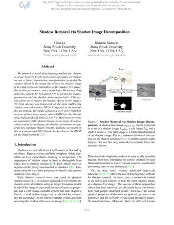
Shadow Removal via Shadow Image DecompositionHieu LeStony Brook UniversityNew York, 11794, USADimitris SamarasStony Brook UniversityNew York, 11794, bstractWe propose a novel deep learning method for shadowremoval. Inspired by physical models of shadow formation,we use a linear illumination transformation to model theshadow effects in the image that allows the shadow imageto be expressed as a combination of the shadow-free image,the shadow parameters, and a matte layer. We use two deepnetworks, namely SP-Net and M-Net, to predict the shadowparameters and the shadow matte respectively. This system allows us to remove the shadow effects on the images.We train and test our framework on the most challengingshadow removal dataset (ISTD). Compared to the state-ofthe-art method, our model achieves a 40% error reductionin terms of root mean square error (RMSE) for the shadowarea, reducing RMSE from 13.3 to 7.9. Moreover, we createan augmented ISTD dataset based on an image decomposition system by modifying the shadow parameters to generate new synthetic shadow images. Training our model onthis new augmented ISTD dataset further lowers the RMSEon the shadow area to 7.4.I relitadwh*I s bowI shadow * α I relit * (1-α)I shadow-freeI shadowα : shadow matte1. IntroductionFigure 1: Shadow Removal via Shadow Image Decomposition. A shadow-free image Ishadow-free can be expressedin terms of a shadow image Ishadow , a relit image Irelit and ashadow matte α. The relit image is a linear transformationof the shadow image. The two unknown factors of this system are the shadow parameters (w, b) and the shadow mattelayer α. We use two deep networks to estimate these twounknown factors.Shadows are cast whenever a light source is blocked byan object. Shadows often confound computer vision algorithms such as segmentation, tracking, or recognition. Theappearance of shadow edges is hard to distinguish fromedges due to material changes [27]. Dark albedo materialregions can be easily misclassified as shadows [18]. Thusmany methods have been proposed to identify and removeshadows from images.Early shadow removal work was based on physicalshadow models [1]. A common approach is to formulate theshadow removal problem using an image formation model,in which the image is expressed in terms of material properties and a light source-occluder system that casts shadows.Hence, a shadow-free image can be obtained by estimating the parameters of the source-occluder system and thenreversing the shadow effects on the image [10, 14, 13, 28].These methods relight the shadows in a physically plausiblemanner. However, estimating the correct solution for suchillumination models is non-trivial and requires considerableprocessing time or user assistance[39, 3].On the other hand, recently published large-scaledatasets [25, 34, 32] allow the use of deep learning methodsfor shadow removal. In these cases, a network is trainedin an end-to-end fashion to map the input shadow imageto a shadow-free image. The success of these approachesshows that deep networks can effectively learn transformations that relight shadowed pixels. However, the actualphysical properties of shadows are ignored, and there is noguarantee that the networks would learn physically plausible transformations. Moreover, there are still well known18578
issues with images generated by deep networks: results tendto be blurry [15, 40] and/or contain artifacts [23]. Howto improve the quality of generated images is an active research topic [16, 35].In this work, we propose a novel method for shadowremoval that takes advantage of both shadow illuminationmodelling and deep learning. Following early shadow removal works, we propose to use a simplified physical illumination model to define the mapping between shadowpixels and their shadow-free counterparts.Our proposed illumination model is a linear transformation consisting of a scaling factor and an additive constant per color channel - for the whole umbra area of the shadow.These scaling factors and additive constants are the parameters of the model, see Fig. 1. The illumination modelplays a key role in our method: with correct parameter estimates, we can use the model to remove shadows from images. We propose to train a deep network (SP-Net) to automatically estimate the parameters of the shadow model.Through training, SP-Net learns a mapping function frominput shadow images to illumination model parameters.Furthermore, we use a shadow matting technique [3, 13,39] to handle the penumbra area of the shadows. We incorporate our illumination model into an image decomposition formulation [24, 3], where the shadow-free imageis expressed as a combination of the shadow image, theparameters of the shadow model, and a shadow densitymatte. This image decomposition formulation allows us toreconstruct the shadow-free image, as illustrated in Fig. 1.The shadow parameters (w, b) represent the transformationfrom the shadowed pixels to the illuminated pixels. Theshadow matte represents the per-pixel linear combinationof the relit image and the shadow image, which results tothe shadow-free image. Previous work often requires userassistance[12] or solving an optimization system [20] to obtain the shadow mattes. In contrast, we propose to train asecond network (M-Net) to accurately predict shadow mattes in a fully automated manner.We train and test our proposed SP-Net and M-Net on theISTD dataset [34], which is the largest and most challenging available dataset for shadow removal. SP-Net alone (nomatting) outperforms the state-of-the-art [12] in shadow removal by 29% in terms of RMSE on shadow areas, from13.3 to 9.5 RMSE. Our full system with both SP-Net andM-Net further improves the overall results by another 17%,which yields a RMSE of 7.9.Our proposed method can realistically modify theshadow effects in the images. First we estimate the shadowparameters and shadow matte from an image. We then addthe shadows back into the shadow-free image with a set ofmodified shadow parameters. As we change the parameters,the shadow effects change accordingly. In this manner, wecan synthetize additional shadow images that serve as aug-mented training data. Training our system on ISTD plus ournewly synthesized images further lowers the RMSE on theshadow areas by 6%, compared to our model trained on theoriginal ISTD dataset.The main contributions of this work are: We propose a new deep learning approach for shadowremoval, grounded by a simplified physical illumination model and an image decomposition formulation. We propose a method for shadow image augmentationbased on our simplified physical illumination modeland the image decomposition formulation. Our proposed method achieves state-of-the-art shadowremoval results on the ISTD dataset.The pre-trained model, shadow removal results, andmore details can be found at: www3.cs.stonybrook.edu/ cvl/projects/SID/index.html2. Related WorksShadow Illumination Models: Early research onshadow removal is motivated by physical modelling of illumination and color [10, 9, 11, 6]. Barrow & Tenenbaum[1] define an intrinsic image algorithm that separates images into the intrinsic components of reflectance and shading. Guo et al. [13] simplify this model to represent the relationship between the shadow pixels and shadow-free pixelsvia a linear system. They estimate the unknown factors viapairing shadow and shadow-free regions. Similarly, Shor &Lischinki [28] propose an illumination model for shadowsin which there is an affine relationship between the lit andshadow intensities at a pixel, including 4 unknown parameters. They define two strips of pixels: one in the shadowedarea and one in the lit area to estimate their parameters.Finlayson et al.[8] create an illuminant-invariant image forshadow detection and removal. Their work is based on aninsight that the shadowed pixels differ from their lit pixelsby a scaling factor. Vicente et al. [31, 33] propose a methodfor shadow removal where they suggest that the color of thelit region can be transferred to the shadowed region via histogram equalization.Shadow Matting: Matting, introduced by Porter & Duff[24], is an effective tool to handle soft shadows. However,it is non-trivial to compute the shadow matte from a singleimage. Chuang et al. [3] use image matting for shadow editing to transfer the shadows between different scenes. Theycompute the shadow matte from a sequence of frames in avideo captured from a static camera. Guo et al. [13] andZhang et al. [39] both use a shadow matte for their shadowremoval frameworks, where they estimate the shadow mattevia the closed-form solution of Levin et al. [20].8579
Deep-Learning Based Shadow Removal: Recentlypublished large-scale datasets [32, 34, 25] enable training deep-learning networks for shadow removal. TheDeshadow-Net of Qu et al. [25] is trained to remove shadows in an end-to-end manner. Their network extracts multicontext features across different layers of a deep networkto predict a shadow matte. This shadow matte is different from ours as it contains both the density and color offset of the shadows. The ST-CGAN proposed by Wang etal. [34] for both shadow detection and removal is a conditional GAN-based framework [15] for shadow detection andremoval. Their framework is trained to predict the shadowmask and shadow-free image in an unified manner, they useGAN losses to improve performance.Inspired by early work, our framework outputs theshadow-free image based on a physically inspired shadowillumination model and a shadow matte. We, however, estimate the parameters of our model and the shadow matte viatwo deep networks in a fully automated manner.3. Shadow and Image Decomposition Model3.1. Shadow Illumination ModelLet us begin by describing our shadow illuminationmodel. We aim to find a mapping function T to transform a shadow pixel Ixshadow to its non-shadow counterpart:Ixshadow-free T (Ixshadow , w) where w are the parameters ofthe model. The form of T has been studied in depth in previous work as discussed in Sec. 2.In this paper, similar to the model of Shor & Lischinski [28], we use a linear function to model the relationshipbetween the lit and shadowed pixels. The intensity of a litpixel is formulated as:Ixshadow-free (λ) Ldx (λ)Rx (λ) Lax (λ)Rx (λ)Ixshadow-free (λ) Ldx (λ)Rx (λ) ax (λ) 1 Ixshadow (λ) (3)We assume that this linear relation is preserved throughout the color acquisition process of the camera [7]. Therefore, we can express the color intensity of the lit pixel x asa linear function of its shadowed value:Ixshadow-free (k) wk Ixshadow (k) bk(4)where Ix (k) represents the value of the pixel x on the image I in color channel k (k R,G,B color channel), bk isthe response of the camera to direct illumination, and wk isresponsible for the attenuation factor of the ambient illumination at this pixel in this color channel. We model eachcolor channel independently to account for possibly different spectral characteristics of the material in shadow as wellas the sensor.We further assume that the two vectors w [wR , wG , wB ] and b [bR , bG , bB ] are constant across allpixels x in the umbra area of the shadow. Under this assumption, we can easily estimate the values of w and b giventhe shadow and shadow-free image using linear regression.We refer to (w, b) as the shadow parameters in the rest ofthe paper.In Sec. 4, we show that we can train a deep-network toestimate these vectors from a single image.3.2. Shadow Image Decomposition SystemWe plug our proposed shadow illumination model intothe following well-known image decomposition system[3, 24, 30, 36]. The system models the shadow-free image using the shadow image, the shadow parameter, and theshadow matte. The shadow-free image can be expressed as:(1)where Ixshadow-free (λ) is the intensity reflected from point xin the scene at wavelength λ, L and R are the illuminationand reflectance respectively, Ld is the direct illuminationand La is the ambient illumination.To cast a shadow on point x, an occluder blocks the direct illumination and a portion of the ambient illuminationthat would otherwise arrive at x. The shadowed intensity atx is:Ixshadow (λ) ax (λ)Lax (λ)Rx (λ)From Eq.1 and 2, we can express the shadow-free pixelas a linear function of the shadowed pixel:(2)where ax (λ) is the attenuation factor indicating the remaining fraction of the ambient illumination that arrives at pointx at wavelength λ. Note that Shor & Lischinski further assume that ax (λ) is the same for all wavelengths λ to simplify their model. This assumption implies that the environment light has the same color from all directions.I shadow-free I shadow · α I relit · (1 α)shadow(5)shadow-freewhere Iand Iare the shadow and shadowfree image respectively, α is the matting layer, and I relit isthe relit image. We define α and I relit below.Each pixel i of the relit image I relit is computed by:Iirelit w · Iishadow b(6)which is the shadow image transformed by the illuminationmodel of Eq. 4. This transformation maps the shadowedpixels to their shadow-free values.The matting layer α represents the per-pixel coefficientsof the linear combination of the relit image and the inputshadow image that results into the shadow-free image. Ideally, the value of α should be 1 at the non-shadow area and0 at the umbra of the shadow area. For the pixels in thepenumbra of the shadow, the value of α gradually changesnear the shadow boundary.8580
I shadowRegressionLossI relitI shadow-free[w, b]M-NetSP-NETshad. matteshad. maskw *I shadow bReconstructionLossFigure 2: Shadow Removal Framework. The shadow parameter estimator network SP-Net takes as input the shadow imageand the shadow mask to predict the shadow parameters (w, b). The relit image I relit is then computed via Eq. 6 using theestimated parameters from SP-Net. The relit image, together with the input shadow image and the shadow mask are theninput into the shadow matte prediction network M-Net to get the shadow matte layer α. The system outputs the shadowfree image via Eq. 5, using the shadow image, the relit image, and the shadow matte. SP-Net learns to predict the shadowparameters (w, b), denoted as the regression loss. M-Net learns to minimize the L1 distance between the output of the systemand the shadow-free image (reconstruction loss).The value of α at pixel i based on the shadow image,shadow-free image, and relit image, follows from Eq. 5 :αi Ii shadow-free Ii relitIi shadow Ii relit(7)We use the image decomposition of Eq. 5 for our shadowremoval framework. The unknown factors are the shadowparameters (w, b) and the shadow matte α. We present ourmethod that uses two deep networks, SP-Net and M-Net,to predict these two factors in the following section. InSec.5.3, we propose a simple method to modify the shadows for an image in order to augment the training data.4. Shadow Removal FrameworkFig. 2 summarizes our framework. The shadow parameter estimator network SP-Net takes as input the shadowimage and the shadow mask to predict the shadow parameters (w, b). The relit image I relit is then computed via Eq.6 with the estimated parameters from SP-Net. The relit image, together with the input shadow image and the shadowmask is then input into the shadow matte prediction networkM-Net to get the shadow matte α. The system outputs theshadow-free image via Eq. 5.4.1. Shadow Parameter Estimator NetworkIn order to recover the illuminated intensity at the shadowed pixel, we need to estimate the parameters of the linear model in Eq. 4. Previous work has proposed differentmethods to estimate the parameters of a shadow illumination model [28, 12, 13, 11, 8, 6]. In this paper, we train SPNet, a deep network model, to directly predict the shadowparameters from the input shadow image.To train SP-Net, we first generate training data. Given atraining pair of a shadow image and a shadow-free image,we estimate the parameters of our linear illumination modelusing a least squares method [4]. For each shadow image,we first erode the shadow mask by 5 pixels in order to define a region that does not contain the partially shadowed(penumbra) pixels. Mapping these shadow pixel values tothe corresponding values in the shadow-free image, givesus a linear regression system, from which we calculate wand b. We compute parameters for each of the three RGBcolor channels and then combine the learned coefficients toform a 6-element vector. This vector is used as the targetedoutput to train SP-Net. The input for SP-Net is the inputshadow image and the associated shadow mask. We trainSP-Net to minimize the L1 distance between the output ofthe network and these computed shadow parameters.We develop SP-Net by customizing a ResNeXt [37]model that is pre-trained on ImageNet [5]. Notice that whilewe use the ground truth shadow mask for training, duringtesting we estimate shadow masks using the shadow detection network proposed by Zhu et al.[41].4.2. Shadow Matte Prediction NetworkOur linear illumination model (Eq. 4) can relight the pixels in the umbra area (fully shadowed). The shadowed pixels in the penumbra (partially shadowed) region are morechallenging as the illumination changes gradually acrossthe shadow boundary [14]. A binary shadow mask cannot model this gradual change. Thus, using a binary maskwithin the decomposition model in Eq. 5 will generate animage with visible boundary artifacts. A solution for this isshadow matting where the soft shadow effects are expressedvia the values of a blending layer.8581
InputRelitShad. MaskUsing S.MaskShad. MatteUsing S.MatteFigure 3: A comparison of the ground truth shadow mask and our shadow matte. From the left to right: The inputimage, the relit image computed from the parameters estimated via SP-Net, the ground truth shadow mask, the final resultswhen we use the shadow mask, the shadow matte computed using our M-Net, and the final shadow-free image when we usethe shadow matte to combine the input and relit image. The matting layer handles the soft shadow and does not generatevisible boundaries in the final result. (Please view in magnification on a digital device to see the difference more clearly.)In this paper, we train a deep network, M-Net, to predict this matting layer. In order to train M-Net, we useEq. 5 to compute the output of our framework where theshadow matte is the output of M-Net. Then the loss functionthat drives the training of M-Net is the L1 distance betweenoutput image and ground truth training shadow-free image,marked as “reconstruction loss” in Fig. 2. This is equivalentto computing the actual value of the shadow matte via Eq.7 and then training M-Net to directly output this value.Fig. 3 illustrates the effectiveness of our shadow matting technique. We show in the figure two shadow removalresults which are computed using a ground-truth shadowmask and a shadow matte respectively. This shadow matteis computed by our model. One can see that using the binary shadow mask to form the shadow-free image createsvisible boundary artifacts as it ignores the penumbra. Theshadow matte from our model captures well the soft shadowand generates an image without shadow boundary artifacts.We design M-Net based on U-Net [26]. The M-Net inputs are the shadow image, the relit image, and the shadowmask. We use the shadow mask as input to M-Net since thematting layer can be considered as a relaxed shadow maskwhere each value represents the strength of the shadow effect at the location rather than just the shadow presence.5. Experiments5.1. Dataset and Evaluation MetricWe train and evaluate on the ISTD dataset [34]. ISTDconsists of image triplets: shadow image, shadow mask,and shadow-free image, captured from different scenes.The training split has 1870 image triplets from 135 scenes,whereas the testing split has 540 triplets from 45 scenes.We notice that the testing set of the ISTD dataset needsto be adjusted since the shadow images and the shadowfree images have inconsistent colors. This is a well knownissue mentioned in the original paper [34]. The reason isthat the shadow and shadow-free image pairs were capturedShad. ImageOriginal GTCorrected GTFigure 4: An example of our color correction method.From left to right: input shadow image, provided shadowfree ground truth image (GT) from ISTD dataset, and theGT image corrected by our method. Comparing to the inputshadow image on the non-shadow area only, the root-meansquare distance of the original GT is 12.9. This value on ourcorrected GT becomes 2.9.at different times of the day which resulted in slightly different environment lights for each image. For example, Fig.4 shows a shadow and shadow-free image pair. The rootmean-square difference between these two images in thenon-shadow area is 12.9. This color inconsistency appearsfrequently in the testing set of the ISTD dataset. On thewhole testing set, the root-mean-square distance betweenthe shadow images and shadow-free images in the nonshadow area is 6.83, as computed by Wang et al.[34].In order to mitigate this color inconsistency, we use linear regression to transform the pixel values in the nonshadow area of each shadow-free image to map into theircounterpart values in the shadow image. We use a linearregression for each color-channel, similar to our methodfor relighting the shadow pixels in Sec. 4.1. This simple transformation transfers the color tone and brightnessof the shadow image to its shadow-free counterpart. Thethird column of Fig. 4 illustrates the effect of our colorcorrection method. Our proposed method reduces the rootmean-square distance between the shadow-free image andthe shadow image from 12.9 to 2.9. The error reduction forthe whole testing set of ISTD goes from 6.83 to 2.6.8582
5.2. Shadow Removal EvaluationWe evaluate our method on the adjusted testing set ofthe ISTD dataset. For metric evaluation we follow [34]and compute the RMSE in the LAB color space on theshadow area, non-shadow area, and the whole image, whereall shadow removal results are re-sized into 256 256 tocompare with the ground truth images at this size. Notethat in contrast to other methods that only output shadowfree images at that resolution, our shadow removal systemworks for input images of any size. Since our method requires shadow masks, we use the model proposed by Zhuet al.[41] pre-trained on the SBU dataset [32] for detecting shadows. We take the model provided by the authorand fine-tune it on the ISTD dataset for 3000 epochs. Thismodel achieves 2.2 Balance Error Rate on the ISTD testing set. To remove the shadow effect in the image, we firstuse SP-Net to compute the shadow parameters (w, b) usingthe input image and the shadow mask computed from theshadow detection network. We use (w, b) to compute a relit image which is input to M-Net, together with the inputimage and the shadow mask to output a matte layer. We obtain the final shadow removal result via Eq. 5. In Table 1,we compare the performance of our method with the recentshadow removal methods of Guo et al.[13], Yang et al.[38],Gong et al.[12], and Wang et al.[34]. All numbers are computed on the adjusted testing images so that they are directlycomparable. The first row shows the numbers for the inputshadow images, i.e. no shadow removal performed.We first evaluate our shadow removal performance using only SP-Net, i.e. we use the binary shadow mask computed by the shadow detector to form the shadow-free image from the shadow image and the relit image. The binaryshadow mask is obtained by simply thresholding the output of the shadow detector with a threshold of 0.95. Asshown in column “SP-Net” (third from the right) in Fig. 8,SP-Net correctly estimates the shadow parameters to relightthe shadow area. Even with visible shadow boundaries, SPNet alone outperforms the previous state-of-the-art, reducing the RMSE on the shadow area by 29%, from 13.3 to9.5.We then evaluate the shadow removal results using bothSP-Net and M-Net, denoted as “SP M-Net” in Tab. 1 andFig. 8. As shown in Fig. 8, the results of M-Net do not contain boundary artifacts. In the third row of Fig. 8, SP-Netoverly relights the shadow area but the shadow matte computed from M-Net effectively corrects these errors. This isbecause M-Net is trained to blend the relit and shadow images to create the shadow-free image. Therefore, M-Netlearns to output a smaller weight for a pixel that is overly litby SP-Net. Using the matte layer of M-Net further reducesthe RMSE on the shadow area by 17%, from 9.5 to 7.9.Overall, our method generates better results than othermethods. Our method does a better job at estimating theInputWang et al.[34]OursGTFigure 5: Comparison of shadow removal between ourmethod and ST-CGAN [34]. ST-CGAN tends to produceblurry images, random artifacts, and incorrect colors of thelit pixels while our method handles all cases well.overall illumination changes compared to the model ofGong et al., which tends to overly relight shadow pixels,as shown in Fig. 8. Our method does not show color inconsistencies within the relit area contrary to all other methods.Fig. 5 qualitatively compares our method and ST-CGAN,which illustrates common issues present in images generated by deep networks [15, 40]. ST-CGAN generally generates blurry images and introduces random artifacts. Ourmethod, albeit not perfect, handles all cases well.Our method fails to recover the shadow-free pixels properly as shown in Fig. 6. The first row, shows how ourmethod overly relights the shadowed area while in the second row, the color of the lit area is incorrect.Finally, we trained and evaluated two alternative designsthat do not require shadow masks as input: (1) The first is anend-to-end shadow-removal system where we jointly train ashadow detector together with our proposed SP-Net and MNet. This framework is harder to train due to the increasein the number of network parameters. (2) The second is aversion of our framework that does not input the shadowmasks into both SP-Net and M-Net. Hence, SP-Net and MNet need to learn to localize the shadow areas implicitly.8583
Table 1: Shadow removal results of our networks compared to state-of-the-art shadow removal methods onthe adjusted ground truth. ( ) The method of Gong etal.[12] is an interactive method that defines the shadow/nonshadow regions via user inputs, thus generates minimal error on the non-shadow area. The metric is RMSE (the lower,the better). Best results are in bold.MethodsShadowNon-ShadowAllInput Image40.22.68.5Yang et al. [38]Guo et al. [13]Wang et al.[34]Gong et al. Net (Ours)SP M-Net (Ours)9.57.93.23.14.13.9Our Method with Alternative SettingsWith a Shad. DetectorNo Input Shadow Mask8.48.35.04.95.55.4Syns. Imagewsyn w 0.8Real ImageSyns. Imagewsyn w 1.7Figure 7: Shadow editing via our decomposition model.We use Eq. 8 to generate synthetic shadow images. As wechange the shadow parameters, the shadow effects changeaccordingly. We show two example images from the ISTDtraining set where in the middle column are the original images and in the first and last column are synthetic.Table 2: Shadow removal results of our networks trainon the augmented ISTD dataset. The metric is RMSE(the lower, the better). Training our framework on the augumented ISTD dataset drops the RMSE on the shadow areafrom 7.9 to 7.4.MethodsTrain. SetShad.Non-Shad.AllSP-NetSP M-NetAug. ISTDAug. ISTD9.07.43.23.14.13.8rameters (w, b), we can form a shadow image by:I shadow I shadow-free · α I darkened · (1 α)InputOursGTFigure 6: Failure cases of our method. In the first row, ourmethod overly lights up the shadow area. In the second row,our method generates incorrect colors.As can be seen in the two bottom rows of Tab. 1, both designs achieved slightly worse shadow removal results thanour main setting.5.3. Dataset Augmentation via Shadow EditingMany deep learning work focus on learning from moreeasily obtainable, weakly-supervised, or synthetic data [2,19, 21, 22, 29, 18, 17]. In this section, we show that wecan modify shadow effects using our proposed illuminationmodel to generate additional training data.Given a shadow matte α, a shadow-free image, and pa-(8)where I darkened has undergone the shadow effect associatedto the set of shadow parameters (w, b). Each pixel i ofI darkened is computed by:Iidarkened (Iishadow-free b) · w 1(9)For each training image, we first compute the shadowparameters and the matte layer via Eqs. 4 and 7. Then, wegenerate a new synthetic shadow image via Eq. 8 with ascaling factor wsyn w k. As seen in Fig. 7, a lowerw leads to an image with a lighter shadow area while ahigher w increases the shadow effects instead. Using thismethod, we augment the ISTD training set by simply choosing k [0.8, 0.9, 1.1, 1.2] to generate a new set of 5320images, which is four times bigger than the original training set. We augment the original ISTD dataset with thisdataset. Training our model on this new augmented ISTDdataset improves our results, as the RMSE drops by 6%,from 7.9 to 7.4, as reported in Tab. 2.8584
InputGuo et al.[13]Yang et al.[38]Gong et al.[12]Wang et al.[34]SP-Net(Ours)SP M-Net(Ours)GroundTruthFigure 8: Comparison of shadow removal on ISTD dataset. Qualitative comparison between our method and previousstate-of-the-art methods: Guo et al.[13], Yang et al.[38], Gong et al.[12], and Wang et al.[34]. “SP-Net” are the shadowremoval results using the parameters computed from SP-Net and a binary shadow mask. “SP M-Net” are the shadowremoval results using the parameters computed from SP-Net and the shadow matte computed from M-Net.6. ConclusionsIn this work, we have presented a novel framework forshadow removal in single images. Our main contributionis to use deep networks as the parameters estimators foran illumination model. Our approach has advantages overpre
shadow detection and removal. Their work is based on an insight that the shadowed pixels differ from their lit pixels by a scaling factor. Vicente et al. [31, 33] propose a method for shadow removal where they suggest that the color of the lit region can be transferred to the shadowed region via his-togram equalization.