WIXLIB

greater than 1 and less than or equal to the maximum number of cases to store in memory. You can set themaximum number of cases to store in memory on the Options tab.Optimization Algorithm. This is the method used to estimate the synaptic weights.Scaled conjugate gradient uses conjugate gradient methods apply only to batch training types, so thismethod is not available for online or mini-batch training.Gradient descent. This method must be used with online or mini-batch training; it can also be used withbatch training.Training Options allow you to fine-tune the optimization algorithm. You generally will not need to changethese settings unless the network runs into problems with estimation. Training options for the scaledconjugate gradient algorithm include: Initial Lambda to specify a number in the interval (0, 0.000001). Initial Sigma to specify a number in the interval (0, 0.0001). Interval Center (a0) and Interval Offset (a) define the interval [a0 a, a0 a], in which weight vectorsare randomly generated when simulated annealing is used. Simulated annealing is used to break out ofa local minimum, with the goal of finding the global minimum, during application of the optimizationalgorithm. This approach is used in weight initialization and automatic architecture selection. Specifya number for the interval center and a number greater than 0 for the interval offset.Training options for the gradient descent algorithm include: Initial Learning Rate. The initial value of the learning rate for the gradient descent algorithm. Ahigher learning rate means that the network will train faster, possibly at the cost of becoming unstable.Specify a number greater than 0. Lower Boundary of Learning Rate. The lower boundary on the learning rate for the gradientdescent algorithm. This setting applies only to online and mini-batch training. Specify a numbergreater than 0 and less than the initial learning rate. Momentum. The initial momentum parameter for the gradient descent algorithm. The momentumterm helps to prevent instabilities caused by a too-high learning rate. Specify a number greater than 0. Learning rate reduction, in Epochs. The number of epochs (p), or data passes of the trainingsample, required to reduce the initial learning rate to the lower boundary of the learning rate whengradient descent is used with online or mini-batch training. This gives you control of the learning ratedecay factor β (1/p K)*ln(η0/ηlow), where η0 is the initial learning rate, ηlow is the lower bound on thelearning rate, and K is the total number of mini-batches (or the number of training records for onlinetraining) in the training dataset. Specify an integer greater than 0.5.Output tabNetwork Structure displays summary informationabout the neural network including the dependentvariables, number of input and output units, numberof hidden layers and units, and activation functions.Diagram displays the network diagram as a noneditable chart. Note that as the number of covariatesand factor levels increases, the diagram becomesmore difficult to interpret.Synaptic weights displays the coefficient estimatesthat show the relationship between the units in agiven layer to the units in the following layer. The synaptic weights are based on the training sample evenif the active dataset is partitioned into training, testing, and holdout data. Note that the number of synapticweights can become rather large and that these weights are generally not used for interpreting networkresults. Network Performance. Displays results used to determine whether the model is "good". Note:Charts in this group are based on the combined training and testing samples or only on the training sampleif there is no testing sample.Instructor:Dr. Prabhat Mittal M. Sc., M.Phil, Ph.D. (FMS, DU)Post-doctoral, University of Minnesota, USAURL:http://people.du.ac.in/ pmittal/5 P a g e

Case processing summary displays the case processing summary table, which summarizes the number ofcases included and excluded in the analysis, in total and by training, testing, and holdout samples.Case Processing ut LayerCovariatesNetwork Information1234Hidden Layer(s)Output LayerPercent485215700150850Number of UnitsaRescaling Method for CovariatesNumber of Hidden LayersNumber of Units in Hidden Layer 1aActivation FunctionDependent VariablesNumber of UnitsActivation FunctionError Function169.3%30.7%100.0%Years with currentemployerDebt to income ratio (x100)Credit card debt inthousandsOther debt in thousands4None12Hyperbolic tangentPreviously defaulted2SoftmaxCross-entropya. Excluding the bias unitThis structure is known as a feed-forward architecture because the connections in the network flowforward from the input layer to the output layer. The input layer contains the predictors. The hidden layercontains unobservable nodes, or units. The value of each hidden unit is some function of the predictors; theexact form of the function is user-controllable specifications. The output layer contains the responses.Since the history of default is a categorical variable with two categories, it is recoded as two indicatorvariables. Each output unit is some function of the hidden units. Again, the exact form of the function isuser-controllable specifications.The MLP network allows a second hidden layer; in that case, each unit of the second hidden layer is afunction of the units in the first hidden layer, and each response is a function of the units in the secondhidden layer.Bias Unit: In a typical artificial neural network each neuron/activity in one "layer" is connected - via aweight - to each neuron in the next activity. Each of these activities stores some sort of computation,normally a composite of the weighted activities in previous layers. A bias unit is an "extra" neuron added toeach pre-output layer that stores the value of 1. Bias units aren't connected to any previous layer and in thissense don't represent a true "activity".Instructor:Dr. Prabhat Mittal M. Sc., M.Phil, Ph.D. (FMS, DU)Post-doctoral, University of Minnesota, USAURL:http://people.du.ac.in/ pmittal/6 P a g e

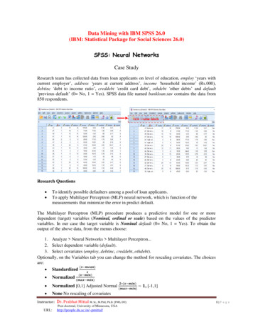
Model summary displays a summary of the neural network results by partition and overall, including theerror, the relative error or percentage of incorrect predictions, the stopping rule used to stop training, andthe training time. The error is the sum-of-squares error when the identity, sigmoid, or hyperbolic tangentactivation function is applied to the output layer. It is the cross-entropy error when the softmax activationfunction is applied to the output layer. Relative errors or percentages of incorrect predictions are displayeddepending on the dependent variable measurement levels. If any dependent variable has scale measurementlevel, then the average overall relative error (relative to the mean model) is displayed. If all dependentvariables are categorical, then the average percentage of incorrect predictions is displayed. Relative errorsor percentages of incorrect predictions are also displayed for individual dependent variables.TrainingTestingModel SummaryCross Entropy Error202.282Percent Incorrect Predictions20.0%Stopping Rule Used1 consecutive step(s) with no decrease in erroraTraining Time0:00:00.19Cross Entropy Error99.585Percent Incorrect Predictions22.3%Dependent Variable: Previously defaulteda. Error computations are based on the testing sample.Classification results displays a classification table for each categorical dependent variable by partition andoverall. Each table gives the number of cases classified correctly and incorrectly for each dependentvariable category. The percentage of the total cases that were correctly classified is also edNoYesOverall PercentNoYesOverall 142417.7%Percent Correct89.4%52.8%80.0%91.1%41.4%77.7%Dependent Variable: Previously defaultedPredicted by observed chart displays a predicted-by-observed-value chart for each dependent variable. Forcategorical dependent variables, clustered boxplots of predicted pseudo-probabilities (an approximation ofjoint probability distribution) are displayed for each response category, with the observed responsecategory as the cluster variable. For scale-dependent variables, a scatterplot is displayed.Instructor:Dr. Prabhat Mittal M. Sc., M.Phil, Ph.D. (FMS, DU)Post-doctoral, University of Minnesota, USAURL:http://people.du.ac.in/ pmittal/7 P a g e

The ROC curve (Receiver Operating Characteristic) is created by plotting the Sensitivity-true positiverate (TPR) also called probability of detection against the (1-specificity)-false positive rate (FPR)probability of false alarm at various threshold settings. It can also be thought of as a plot of the power as afunction of the Type I Error of the decision rule. The ROC curve is thus the sensitivity as a function of fallout.ROC curve displayed for each categorical dependent variable. It also displays a table giving the area undereach curve. For a given dependent variable, the ROC chart displays one curve for each category. If thedependent variable has two categories, then each curve treats the category at issue as the positive stateversus the other category. If the dependent variable hasmore than two categories, then each curve treats thecategory at issue as the positive state versus the aggregateof all other categories.Area Under the CurveAreaPreviously defaultedNo.834Yes.834That is, AUC measures the entire two-dimensional areaunderneath the entire ROC curve from (0,0) to (1,1). Amodel whose predictions are 100% wrong has an AUC of0.0; one whose predictions are 100% correct has an AUCof 1.0. AUC is desirable for the following two reasons: AUC is scale-invariant. It measures how well predictions are ranked, rather than their absolutevalues.AUC is classification-threshold-invariant. It measures the quality of the model's predictionsirrespective of what classification threshold is chosen.Cumulative gains & Lift chart displays a cumulative gains chart for each categorical dependent variable.The display of one curve for each dependent variable category is the same as for ROC curves.Cumulative Gains Chart: The y-axis shows the percentage of % default (yes and no). The x-axis shows the percentage of loan applicants (% total). Baseline (overall response rate): If we contact X% of applicants then receive X% of the responses. Lift Curve: Using the predictions of the response model, calculate the percentage of yes and nodefaults for the percent of loan applicants and map these points to create the lift curve.Lift Chart: Shows the actual lift. Calculate the points on the lift curve by determining the ratio between theresult predicted by our model and the result using no model. For contacting 20% of loan applicant, Gain %20% (Baseline), 28% (No) & 50% (Yes). The y-value of the lift curve at 20% is 50 / 20 2.5 (Yes), 28/201.4 (No).Instructor:Dr. Prabhat Mittal M. Sc., M.Phil, Ph.D. (FMS, DU)Post-doctoral, University of Minnesota, USAURL:http://people.du.ac.in/ pmittal/8 P a g e

Probabilities and Pseudo-ProbabilitiesCategorical dependent variables with softmax activation and cross-entropy error will have a predicted valuefor each category, where each predicted value is the probability that the case belongs to the category.Categorical dependent variables with sum-of-squares error will have a predicted value for each category,but the predicted values cannot be interpreted as probabilities. The procedure saves these predicted pseudoprobabilities even if any are less than 0 or greater than 1, or the sum for a given dependent variable is not 1.The ROC, cumulative gains, and lift charts are created based on pseudo-probabilities. In the event that anyof the pseudo-probabilities are less than 0 or greater than 1, or the sum for a given variable is not 1, they arefirst rescaled to be between 0 and 1 and to sum to 1. Pseudo-probabilities are rescaled by dividing by theirsum. For example, if a case has predicted pseudo-probabilities of 0.50, 0.60, and 0.40 for a three-categorydependent variable, then each pseudo-probability is divided by the sum 1.50 to get 0.33, 0.40, and 0.27. Ifany of the pseudo-probabilities are negative, then the absolute value of the lowest is added to all pseudoprobabilities before the above rescaling. For example, if the pseudo-probabilities are -0.30, 0.50, and 1.30,then first add 0.30 to each value to get 0.00, 0.80, and 1.60. Next, divide each new value by the sum 2.40 toget 0.00, 0.33, and 0.67.6.Save tab is used to save predictions as variables in thedataset.Save predicted value or category for each dependentvariable saves the predicted value for scale-dependentvariables and the predicted category for categoricaldependent variables.Save predicted pseudo-probability or category for eachdependent variable saves the predicted pseudo-probabilitiesfor categorical dependent variables. A separate variable issaved for each of the first n categories, where n is specifiedin the Categories to Save column.Name of Saved Variables generates automatic name andensures that you keep all of your work.Custom names allow you to discard/replace results fromprevious runs without first deleting the saved variables in the Data Editor.7.Export tab is used to save the synaptic weight estimates foreach dependent variable to an Extensible Markup LanguageXML (Predictive Model Markup Language PMML) file. Youcan use this model file to apply the model information toother data files for scoring purposes.8.OptionsUser-Missing Values. Factors must have valid values for a case to be included in the analysis. Thesecontrols allow you to decide whether user-missing values are treated as valid among factors and categoricaldependent variables.Stopping Rules. These are the rules that determine when to stop training the neural network. Trainingproceeds through at least one data pass. Training can then be stopped according to the following criteria,which are checked in the listed order. In the stopping rule definitions that follow, a step corresponds to adata pass for the online and mini-batch methods and an iteration for the batch method.Instructor:Dr. Prabhat Mittal M. Sc., M.Phil, Ph.D. (FMS, DU)Post-doctoral, University of Minnesota, USAURL:http://people.du.ac.in/ pmittal/9 P a g e

Maximum steps The number of steps to allow beforechecking for a decrease in error. If there is no decrease inerror after the specified number of steps, then trainingstops. Specify an integer greater than 0.Data to use for computing prediction error. Chooseautomatically uses the testing sample if it exists and usesthe training sample otherwise. Note that batch trainingguarantees a decrease in the training sample error aftereach data pass; thus, this option applies only to batchtraining if a testing sample exists. Both training and testdata checks the error for each of these samples; this optionapplies only if a testing sample exits.Note: After each complete data pass, online and minibatch training require an extra data pass in order tocompute the training error. This extra data pass can slowtraining considerably, so it is generally recommended thatyou supply a testing sample and select Chooseautomatically in any case.Maximum training time (minutes) for the algorithm to run ( 0).Maximum Training Epochs (data passes) if exceeds than training stops ( 0).Minimum relative change in training error if the relative change in the training error compared to theprevious step is less than the criterion value then training stops ( 0). For online and mini-batch training,this criterion is ignored if only testing data is used to compute the error.Minimum relative change in training error ratio. Training stops if the ratio of the training error to the errorof the null model is less than the criterion value. The null model predicts the average value for alldependent variables. Specify a number greater than 0. For online and mini-batch training, this criterion isignored if only testing data is used to compute the error.Maximum cases to store in memory. This controls the following settings within the multilayer perceptronalgorithms. Specify an integer greater than 1 In automatic architecture selection, the size of the sample used to determine the networkarchicteture is min(1000, memsize), where memsize is the maximum number of cases to store inmemory.In mini-batch training with automatic computation of the number of mini-batches, the number ofmini-batches is min(max(M/10,2), memsize), where M is the number of cases in the trainingsample.Limitations of Neural NetworksWhile Neural Networks has many advantages like handling of nominal/categorical data with nonlinear functionality, it has also certain limitations: Do not know about distribution of the outcomes Cannot propose the test of equality ‘t’, ‘z’ etc Instructor:Can only cont the number of prediction with real and results in different output withdifferent samples.Dr. Prabhat Mittal M. Sc., M.Phil, Ph.D. (FMS, DU)Post-doctoral, University of Minnesota, USAURL:http://people.du.ac.in/ pmittal/10 P a g e

Data Mining with IBM SPSS 26.0 (IBM: Statistical Package for Social Sciences 26.0) SPSS: Neural Networks Case Study Research team has collected data from loan applicants on level of education, employ 'years with current employer', address 'years at current address', income 'household income' (Rs.000),