WIXLIB

which binaries are malware and which are benignware. Then the algorithms learn to determine whether or not new, previously unseen binariesare malicious or benign. We cover training in more detail later in thischapter.NOTEIn this book, we focus on a class of machine learning algorithms known as supervised machine learning algorithms. To train models using these algorithms,we tell them which examples are malicious and which are benign. Another class ofmachine learning algorithms, unsupervised algorithms, does not require us toknow which examples are malicious or benign in our training set. These algorithmsare much less effective at detecting malicious software and malicious behavior, andwe will not cover them in this book.Testing Machine Learning SystemsOnce you’ve trained your machine learning system, you need to checkhow accurate it is. You do this by running the trained system on data thatyou didn’t train it on and seeing how well it determines whether or not thebinaries are malicious or benign. In security, we typically train our systemson binaries that we gathered up to some point in time, and then we test onbinaries that we saw after that point in time, to measure how well our systemswill detect new malware, and to measure how well our systems will avoid producing false positives on new benignware. Most machine learning researchinvolves thousands of iterations that go something like this: we create amachine learning system, test it, and then tweak it, train it again, and test itagain, until we’re satisfied with the results. I’ll cover testing machine learning systems in detail in Chapter 8.Let’s now discuss how a variety of machine learning algorithms work.This is the hard part of the chapter, but also the most rewarding if you takethe time to understand it. In this discussion, I talk about the unifying ideasthat underlie these algorithms and then move on to each algorithm in detail.Understanding Feature Spaces and Decision BoundariesTwo simple geometric ideas can help you understand all machine learning–based detection algorithms: the idea of a geometrical feature space and theidea of a decision boundary. A feature space is the geometrical space defined bythe features you’ve selected, and a decision boundary is a geometrical structurerunning through this space such that binaries on one side of this boundaryare defined as malware, and binaries on the other side of the boundary aredefined as benignware. When we use a machine learning algorithm to classify files as malicious or benign, we extract features so that we can place thesamples in the feature space, and then we check which side of the decisionboundary the samples are on to determine whether the files are malware orbenignware.This geometrical way of understanding feature spaces and decisionboundaries is accurate for systems that operate on feature spaces of one,two, or three dimensions (features), but it also holds for feature spaces withUnderstanding Machine Learning–Based Malware Detectors   93

millions of dimensions, even though it’s impossible to visualize or conceiveof million-dimensional spaces. We’ll stick to examples with two dimensionsin this chapter to make them easy to visualize, but just remember that realworld security machine learning systems pretty much always use hundreds,thousands, or millions of dimensions, and the basic concepts we discuss ina two-dimensional context hold for real-world systems that have more thantwo dimensions.Let’s create a toy malware detection problem to clarify the idea of adecision boundary in a feature space. Suppose we have a training datasetconsisting of malware and benignware samples. Now suppose we extractthe following two features from each binary: the percentage of the filethat appears to be compressed, and the number of suspicious functionseach binary imports. We can visualize our training dataset as shown inFigure 6-1 (bear in mind I created the data in the plot artificially, forexample purposes).Simple DatasetAmount of compressed data (%)100806040200020406080100Number of suspicious imported function callsFigure 6-1: A plot of a sample dataset we’ll use in this chapter, wheregray dots are benignware and black dots are malwareThe two-dimensional space shown in Figure 6-1, which is defined byour two features, is the feature space for our sample dataset. You can seea clear pattern in which the black dots (the malware) are generally inthe upper-right part of the space. In general, these have more suspiciousimported function calls and more compressed data than the benignware,which mostly inhabits the lower-left part of the plot. Suppose, after viewing this plot, you were asked to create a malware detection system basedsolely on the two features we’re using here. It seems clear that, based onthe data, you can formulate the following rule: if a binary has both a lotof compressed data and a lot of suspicious imported function calls, it’smalware, and if it has neither a lot of suspicious imported calls nor muchcompressed data, it’s benignware.94   Chapter 6

In geometrical terms, we can visualize this rule as a diagonal line thatseparates the malware samples from the benignware samples in the featurespace, such that binaries with sufficient compressed data and imported function calls (defined as malware) are above the line, and the rest of the binaries (defined as benignware) are below the line. Figure 6-2 shows such a line,which we call a decision boundary.Defining a Malware Detection Decision Boundary100iocisnboMalwarerydaunAmount of compressed data (%)De806040200Benignware020406080100Number of suspicious imported function callsFigure 6-2: A decision boundary drawn through our sample dataset,which defines a rule for detecting malwareAs you can see from the line, most of the black (malware) dots are onone side of the boundary, and most of the gray (benignware) samples are onthe other side of the decision boundary. Note that it’s impossible to draw aline that separates all of the samples from one another, because the blackand gray clouds in this dataset overlap one another. But from looking atthis example, it appears we’ve drawn a line that will correctly classify newmalware samples and benignware samples in most cases, assuming they follow the pattern seen in the data in this image.In Figure 6-2, we manually drew a decision boundary through our data.But what if we want a more exact decision boundary and want to do it in anautomated way? This is exactly what machine learning does. In other words,all machine learning detection algorithms look at data and use an automated process to determine the ideal decision boundary, such that there’sthe greatest chance of correctly performing detection on new, previouslyunseen data.Let’s look at the way a real-world, commonly used machine learningalgorithm identifies a decision boundary within the sample data shown inFigure 6-3. This example uses an algorithm called logistic regression.Understanding Machine Learning–Based Malware Detectors   95

Logistic RegressionAmount of compressed data (%)100806040200020406080100Number of suspicious imported function callsFigure 6-3: The decision boundary automatically created by traininga logistic regression modelNotice that we’re using the same sample data we used in the previousplots, where gray dots are benignware and black dots are malware. The linerunning through the center of the plot is the decision boundary that thelogistic regression algorithm learns by looking at the data. On the right sideof the line, the logistic regression algorithm assigns a greater than 50 percent probability that binaries are malware, and on the left side of the line, itassigns a less than 50 percent probability that a binary is malware.Now note the shaded regions of the plot. The dark gray shaded region isthe region where the logistic regression model is highly confident that filesare malware. Any new file the logistic regression model sees that has featuresthat land in this region should have a high probability of being malware. Aswe get closer and closer to the decision boundary, the model has less andless confidence about whether or not binaries are malware or benignware.Logistic regression allows us to easily move the line up into the darker regionor down into the lighter region, depending on how aggressive we want to beabout detecting malware. For example, if we move it down, we’ll catch moremalware, but get more false positives. If we move it up, we’ll catch less malware, but get fewer false positives.I want to emphasize that logistic regression, and all other machinelearning algorithms, can operate in arbitrarily high dimensional featurespaces. Figure 6-4 illustrates how logistic regression works in a slightlyhigher dimensional feature space.In this higher-dimensional space, the decision boundary is not a line,but a plane separating the points in the 3D volume. If we were to move tofour or more dimensions, logistic regression would create a hyperplane,which is an n-dimensional plane-like structure that separates the malwarefrom benignware points in this high dimensional space.96   Chapter 6

3210–1–2–3 –2–1012343210–1–2–3Figure 6-4: A planar decision boundary through ahypothetical three dimensional feature space createdby logistic regressionBecause logistic regression is a relatively simple machine learning algorithm, it can only create simple geometrical decision boundaries such aslines, planes, and higher dimensional planes. Other machine learning algorithms can create decision boundaries that are more complex. Consider, forexample, the decision boundary shown in Figure 6-5, given by the k-nearestneighbors algorithm (which I discuss in detail shortly).K-Nearest NeighborsAmount of compressed data (%)100806040200020406080100Number of suspicious imported function callsFigure 6-5: A decision boundary created by the k-nearest neighborsalgorithmAs you can see, this decision boundary isn’t a plane: it’s a highly irregular structure. Also note that some machine learning algorithms can generateUnderstanding Machine Learning–Based Malware Detectors   97

disjointed decision boundaries, which define some regions of the featurespace as malicious and some regions as benign, even if those regions arenot contiguous. Figure 6-6 shows a decision boundary with this irregularstructure, using a different sample dataset with a more complex pattern ofmalware and benignware in our sample feature space.K-Nearest NeighborsAmount of compressed data (%)100806040200020406080100Number of suspicious imported function callsFigure 6-6: A disjoint decision boundary created by the k-nearestneighbors algorithmEven though the decision boundary is noncontiguous, it’s still commonmachine learning parlance to call these disjoint decision boundaries simply“decision boundaries.” You can use different machine learning algorithmsto express different types of decision boundaries, and this difference inexpressivity is why we might pick one machine learning algorithm overanother for a given project.Now that we’ve explored core machine learning concepts like featurespaces and decision boundaries, let’s discuss what machine learning practitioners call overfitting and underfitting next.What Makes Models Good or Bad: Overfitting andUnderfittingI can’t overemphasize the importance of overfitting and underfitting inmachine learning. Avoiding both cases is what defines a good machinelearning algorithm. Good, accurate detection models in machine learning capture the general trend in what the training data says about whatdistinguishes malware from benignware, without getting distracted bythe outliers or the exceptions that prove the rule.98   Chapter 6

Underfit models ignore outliers but fail to capture the general trend,resulting in poor accuracy on new, previously unseen binaries. Overfitmodels get distracted by outliers in ways that don’t reflect the generaltrend, and they yield poor accuracy on previously unseen binaries.Building machine learning malware detection models is all about capturing the general trend that distinguishes the malicious from the benign.Let’s use the examples of underfit, well fit, and overfit models inFigures 6-7, 6-8, and 6-9 to illustrate these terms. Figure 6-7 shows anunderfit model.Underfit (Doesn’t Capture General Trend)Amount of compressed data (%)100806040200020406080100Number of suspicious imported function callsFigure 6-7: An underfit machine learning modelHere, you can see the black dots (malware) cluster in the upper-rightregion of the plot, and the gray dots (benignware) cluster in the lowerleft. However, our machine learning model simply slices the dots downthe middle, crudely separating the data without capturing the diagonaltrend. Because the model doesn’t capture the general trend, we say that itis underfit.Also note that there are only two shades of certainty that the modelgives in all of the regions of the plot: either the shade is dark gray or it’swhite. In other words, the model is either absolutely certain that pointsin the feature space are malicious or absolutely certain they’re benign.This inability to express certainty correctly is also a reason this model isunderfit.Let’s contrast the underfit model in Figure 6-7 with the well-fit model inFigure 6-8.Understanding Machine Learning–Based Malware Detectors   99

Well-Fit (Captures General Trend)Amount of compressed data (%)100806040200020406080100Number of suspicious imported function callsFigure 6-8: A well-fit machine learning modelIn this case, the model not only captures the general trend in the databut also creates a reasonable model of certainty with respect to its estimateof which regions of the feature space are definitely malicious, definitelybenign, or are in a gray area.Note the decision line running from the top to the bottom of thisplot. The model has a simple theory about what divides the malwarefrom the benignware: a vertical line with a diagonal notch in the middleof the plot. Also note the shaded regions in the plot, which tells us thatthe model is only certain that data in the upper-right part of the plot aremalware, and only certain that binaries in the lower-left corner of the plotare benignware.Finally, let’s contrast the overfit model shown next in Figure 6-9 tothe underfit model you saw in Figure 6-7 as well as the well-fit model inFigure 6-8.The overfit model in Figure 6-9 fails to capture the general trend inthe data. Instead, it obsesses over the exceptions in the data, including thehandful of black dots (malware training examples) that occur in the clusterof gray dots (benign training examples) and draws decision boundariesaround them. Similarly, it focuses on the handful of benignware examplesthat occur in the malware cluster, drawing boundaries around those as well.This means that when we see new, previously unseen binaries that happen to have features that place them close to these outliers, the machinelearning model will think they are malware when they are almost definitelybenignware, and vice versa. In practice, this means that this model won’t beas accurate as it could be.100   Chapter 6

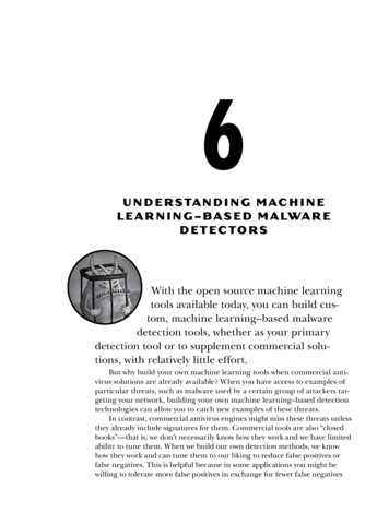
Overfit (Fits to Outliers)Amount of compressed data (%)100806040200020406080100Number of suspicious imported function callsFigure 6-9: An overfit machine learning modelMajor Types of Machine Learning AlgorithmsSo far I’ve discussed machine learning in very general terms, touching ontwo machine learning methods: logistic regression and k-nearest neighbors.In the remainder of this chapter, we delve deeper and discuss logistic regression, k-nearest neighbors, decision trees, and random forest algorithms inmore detail. We use these algorithms quite often in the security data sciencecommunity. These algorithms are complex, but the ideas behind them areintuitive and straightforward.First, let’s look at the sample datasets we use to explore the strengthsand weaknesses of each algorithm, shown in Figure 6-10.I created these datasets for example purposes. On the left, we have oursimple dataset, which I’ve already used in Figures 6-7, 6-8, and 6-9. In thiscase, we can separate the black training examples (malware) from the graytraining examples (benignware) using a simple geometric structure such asa line.The dataset on the right, which I’ve already shown in Figure 6-6, is complex because we can’t separate the malware from the benignware using asimple line. But there is still a clear pattern to the data: we just have to usemore complex methods to create a decision boundary. Let’s see how different algorithms perform with these two sample datasets.Understanding Machine Learning–Based Malware Detectors   101

Amount of compressed data (%)Amount of compressed data (%)Simple Dataset100806040200020406080100Number of suspicious imported function callsComplex Dataset100806040200020406080100Number of suspicious imported function callsFigure 6-10: The two sample datasets we use in this chapter, with black dots representing malware and graydots representing benignwareLogistic RegressionAs you learned previously, logistic regression is a machine learning algorithm that creates a line, plane, or hyperplane (depending on how manyfeatures you provide) that geometrically separates your training malwarefrom your training benignware. When you use the trained model to detectnew malware, logistic regression checks whether a previously unseen binaryis on the malware side or the benignware side of the boundary to determine whether it’s malicious or benign.A limitation of logistic regression is that if your data can’t be separated simply using a line or hyperplane, logistic regression is not the rightsolution. Whether or not you can use logistic regression for your problemdepends on your data and your features. For example, if your problem haslots of individual features that on their own are strong indicators of maliciousness (or “benignness”), then logistic regression might be a winningapproach. If your data is such that you need to use complex relationshipsbetween features to decide that a file is malware, then another approach,like k-nearest neighbors, decision trees, or random forest, might make moresense.To illustrate the strengths and weaknesses of logistic regression, let’slook at the performance of logistic regression on our two sample datasets,as shown in Figure 6-11. We see that logistic regression yields a very effective separation of the malware and benignware in our simple dataset (onthe left). In contrast, the performance of logistic regression on our complex dataset (on the right) is not effective. In this case, the logistic regression algorithm gets confused, because it can only express a linear decisionboundary. You can see both binary types on both sides of the line, and theshaded gray confidence bands don’t really make any sense relative to thedata. For this more complex dataset, we’d need to use an algorithm capableof expressing more geometric structures.102   Chapter 6

Simple Dataset100Amount of compressed data (%)Amount of compressed data (%)Logistic Regression806040200020406080100Number of suspicious imported function callsComplex Dataset100806040200020406080100Number of suspicious imported function callsFigure 6-11: A decision boundary drawn through our sample datasets using logistic regressionThe Math Behind Logistic RegressionLet’s now look at the math behind how logistic regression detects malwaresamples. Listing 6-1 shows Pythonic pseudocode for computing the probability that a binary is malware using logistic regression.def logistic regression(compressed data, suspicious calls, learned parameters): ucompressed data compressed data * learned parameters["compressed data weight"] suspicious calls suspicious calls * learned parameters["suspicious calls weight"]score compressed data suspicious calls bias wreturn logistic function(score)def logistic function(score): xreturn 1/(1.0 math.e**(-score))Listing 6-1: Pseudocode using logistic regression to calculate probabilityLet’s step through the code to understand what this means. We firstdefine the logistic regression function and its parameters. Its parametersare the features of the binary (compressed data and suspicious calls) that represent the amount of compressed data and the number of suspicious callsit makes, respectively, and the parameter learned parameters stands for theelements of the logistic regression function that were lea

machine learning systems in Python in Chapter 8. Let's get started. Steps for Building a Machine learning-Based Detector There is a fundamental difference between machine learning and other kinds of computer algorithms. Whereas traditional algorithms tell the com-puter what to do, machine-learning systems learn how to solve a problem by .