WIXLIB

Machine-Learning-Course Documentation, Release 1.0Typically the holdout method involves splitting a dataset into 20-30% test data and the rest as training data. Thesenumbers can vary - a larger percentage of test data will make your model more prone to errors as it has less trainingexperience, while a smaller percentage of test data may give your model an unwanted bias towards the training data.This lack of training or bias can lead to Underfitting/Overfitting of our model.2.3 K-Fold Cross ValidationK-Fold Cross Validation helps remove these biases from your model by repeating the holdout method on k subsets ofyour dataset. With K-Fold Cross Validation, a dataset is broken up into several unique folds of test and training data.The holdout method is performed using each combination of data, and the results are averaged to find a total errorestimation.A “fold” here is a unique section of test data. For instance, if you have 100 data points and use 10 folds, each foldcontains 10 test points. K-Fold Cross Validation is important because it allows you to use your complete dataset forboth training and testing. It’s especially useful when evaluating a model using small or limited datasets.2.4 Leave-P-Out / Leave-One-Out Cross ValidationLeave-P-Out Cross Validation (LPOCV) tests a model by using every possible combination of P test data points on amodel. As a simple example, if you have 4 data points and use 2 test points, the model will be trained and tested ere “T” is a test point, and “-” is a training point. Below is another visualization of LPOCV:LPOCV can provide an extremely accurate error estimation, but can quickly become exhaustive for large datasets.The amount of testing iterations a model has to go through using LPOCV can be calculated using a mathematicalcombination n C P, with n being our total number of data points. We can see, for instance, that a LPOCV run using adataset of 10 points with 3 test points would require 10 C 3 120 iterations.4Chapter 2. Cross-Validation

Machine-Learning-Course Documentation, Release 1.0Fig. 1: Ref: ategies/2.4. Leave-P-Out / Leave-One-Out Cross Validation5

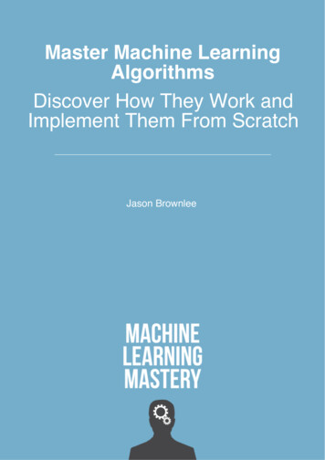
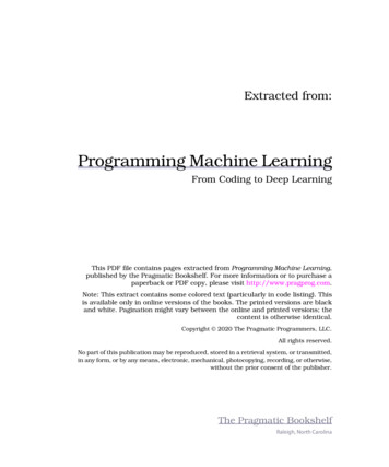
Machine-Learning-Course Documentation, Release 1.0Because of this, Leave-One-Out Cross Validation (LOOCV) is a commonly used cross-validation method. It is just asubset of LPOCV, with P being 1. This allows us to evaluate a model in the same number of steps as there are datapoints. LOOCV can also be seen as K-Fold Cross Validation, where the number of folds is equal to the number of datapoints.Fig. 2: Ref: ategies/Similar to K-Fold Cross Validation, LPOCV and LOOCV train a model using the full dataset. They are particularlyuseful when you’re working with a small dataset, but incur performance tradeoffs.2.5 ConclusionCross-validation is a way to validate your model against new data. The most effective forms of cross-validation involverepeatedly testing a model against a dataset until every point or combination of points have been used to validate amodel, though this comes with performance trade-offs. We discussed several methods of splitting a dataset for crossvalidation: Holdout Method: Splitting a percent of data off as test data K-Fold Method: Dividing data into sections, using each as a test/train split Leave-P-Out Method: Using every combination of a number of points (P) as test data2.6 MotivationThere are many different types of machine learning models, including Linear/Logistic Regression, K-NearestNeighbors, and Support Vector Machines - but how do we know which type of model is the best for our dataset?Using a model unsuitable for our data will lead to less accurate predictions, and could lead to financial, physical, orother forms of harm. Individuals and companies should make sure to cross-validate any models they put into use.2.7 Code ExamplesThe provided code shows how to split a set of data with the three discussed methods of cross-validation using ScikitLearn, a Python machine learning library.6Chapter 2. Cross-Validation

Machine-Learning-Course Documentation, Release 1.0holdout.py splits a set of sample diabetes data using the Holdout Method. In scikit-learn, this is done using a functioncalled train test split() which randomly splits a set of data into two portions:TRAIN SPLIT 0.7.dataset datasets.load diabetes().x train, x test, y train, y test train test split(.)Note that you can change the portion of data used for training by changing the TRAIN SPLIT value at the top. Thisshould be a number from 0 to 1. Output from this file shows the number of training and test points used for the split. Itmay be beneficial to see the actual data points - if you would like to see these, uncomment the last two print statementsin the script.k-fold.py splits a set of data using the K-Fold Method. This is done by creating a KFold object initialized with thenumber of splits to use. Scikit-learn makes it easy to split data by calling KFold’s split() method:NUM SPLITS 3data numpy.array([[1, 2], [3, 4], [5, 6], [7, 8], [9, 10], [11, 12]])kfold KFold(n splits NUM SPLITS)split data kfold.split(data)The return value of this is an array of train and test points. Note that you can play with the number of splits by changingthe associated value at the top of the script. This script not only outputs the train/test data, but also outputs a nice barwhere where you can track the progress of the current fold:[ T T - - - - ]Train: (2: [5 6]) (3: [7 8]) (4: [ 9 10]) (5: [11 12])Test: (0: [1 2]) (1: [3 4]).leave-p-out.py splits a set of data using both the Leave-P-Out and Leave-One-Out Methods. This is done by creatingLeavePOut/LeaveOneOut objects, the LPO initialized with the number of splits to use. Similar to KFold, the train-testdata split is created with the split() method:P VAL 2data numpy.array([[1, 2], [3, 4], [5, 6], [7, 8]])loocv LeaveOneOut()lpocv LeavePOut(p P VAL)split loocv loocv.split(data)split lpocv lpocv.split(data)Note that you can change the P value at the top of the script to see how different values operate.2.8 References1. -machine-learning-72924a69872f2.8. References7

Machine-Learning-Course Documentation, Release 1.02. lidation/3. machine-learning4. ategies/8Chapter 2. Cross-Validation

CHAPTER3Linear Regression Motivation Overview When to Use Cost Function Methods– Ordinary Least Squares– Gradient Descent Code Conclusion References3.1 MotivationWhen we are presented with a data set, we try and figure out what it means. We look for connections between the datapoints and see if we can find any patterns. Sometimes those patterns are hard to see so we use code to help us findthem. There are lots of different patterns data can follow so it helps if we can narrow down those options and writeless code to analyze them. One of those patterns is a linear relationship. If we can find this pattern in our data, we canuse the linear regression technique to analyze it.9

Machine-Learning-Course Documentation, Release 1.03.2 OverviewLinear regression is a technique used to analyze a linear relationship between input variables and a single outputvariable. A linear relationship means that the data points tend to follow a straight line. Simple linear regressioninvolves only a single input variable. Figure 1 shows a data set with a linear relationship.Fig. 1: Figure 1. A sample data set with a linear relationship [code]Our goal is to find the line that best models the path of the data points called a line of best fit. The equation in Equation1, is an example of a linear equation.Fig. 2: Equation 1. A linear equationFigure 2 shows the data set we use in Figure 1 with a line of best fit through it.Let’s break it down. We already know that x is the input value and y is our predicted output. a0 and a1 describe theshape of our line. a0 is called the bias and a1 is called a weight. Changing a0 will move the line up or down on theplot and changing a1 changes the slope of the line. Linear regression helps us pick appropriate values for a0 and a1 .Note that we could have more than one input variable. In this case, we call it multiple linear regression. Addingextra input variables just means that we’ll need to find more weights. For this exercise, we will only consider a simplelinear regression.10Chapter 3. Linear Regression

Machine-Learning-Course Documentation, Release 1.0Fig. 3: Figure 2. The data set from Figure 1 with a line of best fit [code]3.2. Overview11

Machine-Learning-Course Documentation, Release 1.03.3 When to UseLinear regression is a useful technique but isn’t always the right choice for your data. Linear regression is a goodchoice when there is a linear relationship between your independent and dependent variables and you are trying topredict continuous values [Figure 1].It is not a good choice when the relationship between independent and dependent variables is more complicated orwhen outputs are discrete values. For example, Figure 3 shows a data set that does not have a linear relationship solinear regression would not be a good choice.Fig. 4: Figure3. A sample data set without a linear relationship [code]It is worth noting that sometimes you can apply transformations to data so that it appears to be linear. For example,you could apply a logarithm to exponential data to flatten it out. Then you can use linear regression on the transformeddata. One method of transforming data in sklearn is documented here.Figure 4 is an example of data that does not look linear but can be transformed to have a linear relationship.Figure 5 is the same data after transforming the output variable with a logarithm.3.4 Cost FunctionOnce we have a prediction, we need some way to tell if it’s reasonable. A cost function helps us do this. The costfunction compares all the predictions against their actual values and provides us with a single number that we can use12Chapter 3. Linear Regression

Machine-Learning-Course Documentation, Release 1.0Fig. 5: Figure 4. A sample data set that follows an exponential curve [code]3.4. Cost Function13

Machine-Learning-Course Documentation, Release 1.0Fig. 6: Figure 5. The data set from Figure 4 after applying a logarithm to the output variable [code]14Chapter 3. Linear Regression

Machine-Learning-Course Documentation, Release 1.0to score the prediction function. Figure 6 shows the cost for one such prediction.Fig. 7: Figure 6. The plot from Figure 2 with the cost of one prediction emphasized [code]Two common terms that appear in cost functions are the error and squared error. The error [Equation 2] is how faraway from the actual value our prediction is.Fig. 8: Equation 2. An example error functionSquaring this value gives us a useful expression for the general error distance as shown in Equation 3.Fig. 9: Equation 3. An example squared error functionWe know an error of 2 above the actual value and an error of 2 below the actual value should be about as bad as eachother. The squared error makes this clear because both of these values result in a squared error of 4.We will use the Mean Squared Error (MSE) function shown in Equation 4 as our cost function. This function finds theaverage squared error value for all of our data points.Cost functions are important to us because they measure how accurate our model is against the target values. Makingsure our models are accurate will remain a key theme throughout later modules.3.4. Cost Function15

Machine-Learning-Course Documentation, Release 1.0Fig. 10: Equation 4. The Mean Squared Error (MSE) function3.5 MethodsA lower cost function means a lower average error across the data points. In other words, lower cost means a moreaccurate model for the data set. We will briefly mention a couple of methods for minimizing the cost function.3.5.1 Ordinary Least SquaresOrdinary least squares is a common method for minimizing the cost function. In this method, we treat the data as onebig matrix and use linear algebra to estimate the optimal values of the coefficients in our linear equation. Luckily, youdon’t have to worry about doing any linear algebra because the Python code handles it for you. This also happens tobe the method used for this modules code.Below are the relevant lines of Python code from this module related to ordinary least squares.# Create a linear regression objectregr linear model.LinearRegression()3.5.2 Gradient DescentGradient descent is an iterative method of guessing the coefficients of our linear equation in order to minimize thecost function. The name comes from the concept of gradients in calculus. Basically this method will slightly movethe values of the coefficients and monitor whether the cost decreases or not. If the cost keeps increasing over severaliterations, we stop because we’ve probably hit the minimum already. The number of iterations and tolerance beforestopping can both be chosen to fine tune the method.Below are the relevant lines of Python code from this module modified to use gradient descent.# Create a linear regression objectregr linear model.SGDRegressor(max iter 10000, tol 0.001)3.6 CodeThis module’s main code is available in the linear regression lobf.py file.All figures in this module were created with simple modifications of the linear regression.py code.In the code, we analyze a data set with a linear relationship. We split the data into a training set to train our modeland a testing set to test its accuracy. You may have guessed that the model used is based on linear regression. We alsodisplay a nice plot of the data with a line of best fit.3.7 ConclusionIn this module, we learned about linear regression. This technique helps us model data with linear relationships. Linearrelationships are fairly simple but still show up in a lot of data sets so this is a good technique to know. Learning about16Chapter 3. Linear Regression

Machine-Learning-Course Documentation, Release 1.0linear regression is a good first step towards learning more complicated analysis techniques. We will build on a lot ofthe concepts covered here in later modules.3.8 References1. https://towardsdatascience.com/

Machine learning tools are now available through the Cloud and on large scale distributed systems. 1.1.2Why is machine learning important? Machine learning has practical applications for a range of common business problems. By using machine learning, organizations can complete tasks in less time and more efficiently.