Transcription
Decision Trees—What Are They?Introduction . 1Using Decision Trees with Other Modeling Approaches . 5Why Are Decision Trees So Useful? . 8Level of Measurement . 11IntroductionDecision trees are a simple, but powerful form of multiple variable analysis. Theyprovide unique capabilities to supplement, complement, and substitute for traditional statistical forms of analysis (such as multiple linear regression) a variety of data mining tools and techniques (such as neural networks) recently developed multidimensional forms of reporting and analysis found in thefield of business intelligence
2 Decision Trees for Business Intelligence and Data Mining: Using SAS Enterprise MinerDecision trees are produced by algorithms that identify various ways of splitting a dataset into branch-like segments. These segments form an inverted decision tree thatoriginates with a root node at the top of the tree. The object of analysis is reflected in thisroot node as a simple, one-dimensional display in the decision tree interface. The name ofthe field of data that is the object of analysis is usually displayed, along with the spread ordistribution of the values that are contained in that field. A sample decision tree isillustrated in Figure 1.1, which shows that the decision tree can reflect both a continuousand categorical object of analysis. The display of this node reflects all the data setrecords, fields, and field values that are found in the object of analysis. The discovery ofthe decision rule to form the branches or segments underneath the root node is based on amethod that extracts the relationship between the object of analysis (that serves as thetarget field in the data) and one or more fields that serve as input fields to create thebranches or segments. The values in the input field are used to estimate the likely value inthe target field. The target field is also called an outcome, response, or dependent field orvariable.The general form of this modeling approach is illustrated in Figure 1.1. Once therelationship is extracted, then one or more decision rules can be derived that describe therelationships between inputs and targets. Rules can be selected and used to display thedecision tree, which provides a means to visually examine and describe the tree-likenetwork of relationships that characterize the input and target values. Decision rules canpredict the values of new or unseen observations that contain values for the inputs, butmight not contain values for the targets.
Chapter 1: Decision Trees—What Are They?3Figure 1.1: Illustration of the Decision TreeEach rule assigns a record or observation from the data set to a node in a branch orsegment based on the value of one of the fields or columns in the data set.1 Fields orcolumns that are used to create the rule are called inputs. Splitting rules are applied oneafter another, resulting in a hierarchy of branches within branches that produces thecharacteristic inverted decision tree form. The nested hierarchy of branches is called a1The SAS Enterprise Miner decision tree contains a variety of algorithms to handle missing values, includinga unique algorithm to assign partial records to different segments when the value in the field that is beingused to determine the segment is missing.
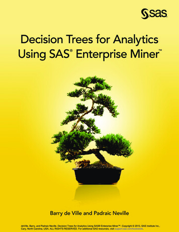
4 Decision Trees for Business Intelligence and Data Mining: Using SAS Enterprise Minerdecision tree, and each segment or branch is called a node. A node with all its descendentsegments forms an additional segment or a branch of that node. The bottom nodes of thedecision tree are called leaves (or terminal nodes). For each leaf, the decision ruleprovides a unique path for data to enter the class that is defined as the leaf. All nodes,including the bottom leaf nodes, have mutually exclusive assignment rules; as a result,records or observations from the parent data set can be found in one node only. Once thedecision rules have been determined, it is possible to use the rules to predict new nodevalues based on new or unseen data. In predictive modeling, the decision rule yields thepredicted value.Figure 1.2: Illustration of Decision Tree Nomenclature
Chapter 1: Decision Trees—What Are They?5Although decision trees have been in development and use for over 50 years (one of theearliest uses of decision trees was in the study of television broadcasting by Belson in1956), many new forms of decision trees are evolving that promise to provide excitingnew capabilities in the areas of data mining and machine learning in the years to come.For example, one new form of the decision tree involves the creation of random forests.Random forests are multi-tree committees that use randomly drawn samples of data andinputs and reweighting techniques to develop multiple trees that, when combined,provide for stronger prediction and better diagnostics on the structure of the decision tree.Besides modeling, decision trees can be used to explore and clarify data for dimensionalcubes that can be found in business analytics and business intelligence.Using Decision Trees with Other Modeling ApproachesDecision trees play well with other modeling approaches, such as regression, and can beused to select inputs or to create dummy variables representing interaction effects forregression equations. For example, Neville (1998) explains how to use decision trees tocreate stratified regression models by selecting different slices of the data population forin-depth regression modeling.The essential idea in stratified regression is to recognize that the relationships in the dataare not readily fitted for a constant, linear regression equation. As illustrated in Figure1.3, a boundary in the data could suggest a partitioning so that different regressionmodels of different forms can be more readily fitted in the strata that are formed byestablishing this boundary. As Neville (1998) states, decision trees are well suited inidentifying regression strata.
6 Decision Trees for Business Intelligence and Data Mining: Using SAS Enterprise MinerFigure 1.3: Illustration of the Partitioning of Data Suggesting StratifiedRegression ModelingDecision trees are also useful for collapsing a set of categorical values into ranges that arealigned with the values of a selected target variable or value. This is sometimes calledoptimal collapsing of values. A typical way of collapsing categorical values togetherwould be to join adjacent categories together. In this way 10 separate categories can bereduced to 5. In some cases, as illustrated in Figure 1.4, this results in a significantreduction in information. Here categories 1 and 2 are associated with extremely low andextremely high levels of the target value. In this example, the collapsed categories 3 and4, 5 and 6, 7 and 8, and 9 and 10 work better in this type of deterministic collapsingframework; however, the anomalous outcome produced by collapsing categories 1 and 2together should serve as a strong caution against adopting any such scheme on a regularbasis.Decision trees produce superior results. The dotted lines show how collapsing thecategories with respect to the levels of the target yields different and better results. If weimpose a monotonic restriction on the collapsing of categories—as we do when werequest tree growth on the basis of ordinal predictors—then we see that category 1becomes a group of its own. Categories 2, 3, and 4 join together and point to a relatively
Chapter 1: Decision Trees—What Are They?7high level in the target. Categories 5, 6, and 7 join together to predict the lowest level ofthe target. And categories 8, 9, and 10 form the final group.If a completely unordered grouping of the categorical codes is requested—as would bethe case if the input was defined as “nominal”—then the 3 bins as shown in the bottom ofFigure 1.4 might be produced. Here the categories 1, 5, 6, 7, 9, and 10 group together asassociated with the highest level of the target. The medium target levels produce agrouping of categories 3, 4, and 8. The lone high target level that is associated withcategory 2 falls out as a category of its own.Figure 1.4: Illustration of Forming Nodes by Binning Input-Target Relationships
8 Decision Trees for Business Intelligence and Data Mining: Using SAS Enterprise MinerSince a decision tree allows you to combine categories that have similar values withrespect to the level of some target value there is less information loss in collapsingcategories together. This leads to improved prediction and classification results. Asshown in the figure, it is possible to intuitively appreciate that these collapsed categoriescan be used as branches in a tree. So, knowing the branch—for example, branch 3(labeled BIN 3), we are better able to guess or predict the level of the target. In the caseof branch 2 we can see that the target level lies in the mid-range, whereas in the lastbranch—here collapsed categories 1, 5, 6, 7, 9, 10—the target is relatively low.Why Are Decision Trees So Useful?Decision trees are a form of multiple variable (or multiple effect) analyses. All forms ofmultiple variable analyses allow us to predict, explain, describe, or classify an outcome(or target). An example of a multiple variable analysis is a probability of sale or thelikelihood to respond to a marketing campaign as a result of the combined effects ofmultiple input variables, factors, or dimensions. This multiple variable analysis capabilityof decision trees enables you to go beyond simple one-cause, one-effect relationships andto discover and describe things in the context of multiple influences. Multiple variableanalysis is particularly important in current problem-solving because almost all criticaloutcomes that determine success are based on multiple factors. Further, it is becomingincreasingly clear that while it is easy to set up one-cause, one-effect relationships in theform of tables or graphs, this approach can lead to costly and misleading outcomes.According to research in cognitive psychology (Miller 1956; Kahneman, Slovic, andTversky 1982) the ability to conceptually grasp and manipulate multiple chunks ofknowledge is limited by the physical and cognitive processing limitations of the shortterm memory portion of the brain. This places a premium on the utilization ofdimensional manipulation and presentation techniques that are capable of preserving andreflecting high-dimensionality relationships in a readily comprehensible form so that therelationships can be more easily consumed and applied by humans.There are many multiple variable techniques available. The appeal of decision trees liesin their relative power, ease of use, robustness with a variety of data and levels ofmeasurement, and ease of interpretability. Decision trees are developed and presentedincrementally; thus, the combined set of multiple influences (which are necessary to fullyexplain the relationship of interest) is a collection of one-cause, one-effect relationships
Chapter 1: Decision Trees—What Are They?9presented in the recursive form of a decision tree. This means that decision trees dealwith human short-term memory limitations quite effectively and are easier to understandthan more complex, multiple variable techniques. Decision trees turn raw data into anincreased knowledge and awareness of business, engineering, and scientific issues, andthey enable you to deploy that knowledge in a simple, but powerful set of humanreadable rules.Decision trees attempt to find a strong relationship between input values and target valuesin a group of observations that form a data set. When a set of input values is identified ashaving a strong relationship to a target value, then all of these values are grouped in a binthat becomes a branch on the decision tree. These groupings are determined by theobserved form of the relationship between the bin values and the target. For example,suppose that the target average value differs sharply in the three bins that are formed bythe input. As shown in Figure 1.4, binning involves taking each input, determining howthe values in the input are related to the target, and, based on the input-target relationship,depositing inputs with similar values into bins that are formed by the relationship.To visualize this process using the data in Figure 1.4, you see that BIN 1 contains values1, 5, 6, 7, 9, and 10; BIN 2 contains values 3, 4, and 8; and BIN 3 contains value 2. Thesort-selection mechanism can combine values in bins whether or not they are adjacent toone another (e.g., 3, 4, and 8 are in BIN 2, whereas 7 is in BIN 1). When only adjacentvalues are allowed to combine to form the branches of a decision tree, then theunderlying form of measurement is assumed to monotonically increase as the numericcode of the input increases. When non-adjacent values are allowed to combine, then theunderlying form of measurement is non-monotonic. A wide variety of different forms ofmeasurement, including linear, nonlinear, and cyclic, can be modeled using decisiontrees.A strong input-target relationship is formed when knowledge of the value of an inputimproves the ability to predict the value of the target. A strong relationship helps youunderstand the characteristics of the target. It is normal for this type of relationship to beuseful in predicting the values of targets. For example, in most animal populations,knowing the height or weight improves the ability to predict the gender. In the followingdisplay, there are 28 observations in the data set. There are 20 males and 8 females.
10 Decision Trees for Business Intelligence and Data Mining: Using SAS Enterprise MinerGenderWeightHeightHt 841171631942012542012062162062201824’105’ 45’ eheavyheavyheavyheavyheavyheavyheavyheavyIn this display, the overall average height is 5’6 and the overall average weight is 183.Among males, the average height is 5’7, while among females, the average height is 5’3(males weigh 200 on average, versus 155 for females).Knowing the gender puts us in a better position to predict the height and weight of theindividuals, and knowing the relationship between gender and height and weight puts usin a better position to understand the characteristics of the target. Based on therelationship between height and weight and gender, you can infer that females are bothsmaller and lighter than males. As a result, you can see how this sort of knowledge that isbased on gender can be used to determine the height and weight of unseen humans.From the display, you can construct a branch with three leaves to illustrate how decisiontrees are formed by grouping input values based on their relationship to the target.
Chapter 1: Decision Trees—What Are They?11Figure 1.5: Illustration of Decision Tree Partitioning of Physical MeasurementsRoot NodeAverage Weight: 183 lbLow weightAverage: 138 lbMedium weightAverage: 183 lbHeavy weightAverage: 227 lbLevel of MeasurementThe example as shown here illustrates an important characteristic of decision trees: bothquantitative and qualitative data can be accommodated in decision tree construction.Quantitative data, like height and weight, refers to quantities that can be manipulatedwith arithmetic operations such as addition, subtraction, and multiplication. Qualitativedata, such as gender, cannot be used in arithmetic operations, but can be presented intables or decision trees. In the previous example, the target field is weight and ispresented as an average. Height, BMIndex, or BodyType could have been used as inputsto form the decision tree.Some data, such as shoe size, behaves like both qualitative and quantitative data. Forexample, you might not be able to do meaningful arithmetic with shoe size, even thoughthe sequence of numbers in shoe sizes is in an observable order. For example, with shoesize, size 10 is larger than size 9, but it is not twice as large as size 5.Figure 1.6 displays a decision tree developed with a categorical target variable. Thisfigure shows the general, tree-like characteristics of a decision tree and illustrates howdecision trees display multiple relationships—one branch at a time. In subsequent figures,decision trees are shown with continuous or numeric fields as targets. This shows howdecision trees are easily developed using targets and inputs that are both qualitative(categorical data) and quantitative (continuous, numeric data).
12 Decision Trees for Business Intelligence and Data Mining: Using SAS Enterprise MinerFigure 1.6: Illustration of a Decision Tree with a Categorical TargetThe decision tree in Figure 1.6 displays the results of a mail-in customer surveyconducted by HomeStuff, a national home goods retailer. In the survey, customers hadthe option to enter a cash drawing. Those who entered the drawing were classified as aHomeStuff best customer. Best customers are coded with 1 in the decision tree.The top-level node of the decision tree shows that, of the 8399 respondents to the survey,57% were classified as best customers, while 43% were classified as other (codedwith 0).Figure 1.6 shows the general characteristics of a decision tree, such as partitioning theresults of a 1–0 (categorical) target across various input fields in the customer surveydata set. Under the top-level node, the field GENDER further characterizes the best –other (1–0) response. Females (coded with F) are more likely to be best customers thanmales (coded with M). Fifty-nine percent of females are best customers versus fifty-fourpercent of males. A wide variety of splitting techniques has been developed over time togauge whether this difference is statistically significant and whether the results areaccurate and reproducible. In Figure 1.6, the difference between males and females isstatistically significant. Whether a difference of 5% is significant from a business point ofview is a question that is best answered by the business analyst.
Chapter 1: Decision Trees—What Are They?13The splitting techniques that are used to split the 1–0 responses in the data set are used toidentify alternative inputs (for example, income or purchase history) for gender. Thesetechniques are based on numerical and statistical techniques that show an improvementover a simple, uninformed guess at the value of a target (in this example, best–other), aswell as the reproducibility of this improvement with a new set of data.Knowing the gender enables us to guess that females are 5% more likely to be a bestcustomer than males. You could set up a separate, independent hold out or validation dataset and (having determined that the gender effect is useful or interesting) you might seewhether the strength and direction of the effect is reflected in the hold out or validationdata set. The separate, independent data set will show the results if the decision tree isapplied to a new data set, which indicates the generality of the results. Another way toassess the generality of the results is to look at data distributions that have been studiedand developed by statisticians who know the properties of the data and who havedeveloped guidelines based on the properties of the data and data distributions. Theresults could be compared to these data distributions and, based on the comparisons, youcould determine the strength and reproducibility of the results. These approaches arediscussed at greater length in Chapter 3, “The Mechanics of Decision Tree Construction.”Under the female node in the decision tree in Figure 1.6, female customers can be furthercategorized into best–other categories based on the total lifetime visits that they havemade to HomeStuff stores: those who have made fewer than 3.5 visits are less likely to bebest customers compared to those who have made more than 4.5 visits: 29% versus100%. (In the survey, a shopping visit of less than 20 minutes was characterized as a halfvisit.)On the right side of the figure, the decision tree is asymmetric; a new field—Net sales—has entered the analysis. This suggests that Net sales is a stronger or more relevantpredictor of customer status than Total lifetime visits, which was used to analyzefemales. It was this kind of asymmetry that spurred the initial development of decisiontrees in the statistical community: these kinds of results demonstrate the importance ofthe combined (or interactive) effect of two indicators in displaying the drivers of anoutcome. In the case of males, when Net sales exceed 281.50, then the likelihood ofbeing a best customer increases from 45% to 77%.As shown in the asymmetry of the decision tree, female behavior and male behavior havedifferent nuances. To explain or predict female behavior, you have to look at theinteraction of gender (in this case, female) with Total lifetime visits. For males, Netsales is an important characteristic to look at.
14 Decision Trees for Business Intelligence and Data Mining: Using SAS Enterprise MinerIn Figure 1.6, of all the k-way or n-way branches that could have been formed in thisdecision tree, the 2-way branch is identified as best. This indicates that a 2-way branchproduces the strongest effect. The strength of the effect is measured through a criterionthat is based on strength of separation, statistical significance, or reproducibility, withrespect to a validation process. These measures, as applied to the determination of branchformation and splitting criterion identification, are discussed further in Chapter 3.Decision trees can accommodate categorical (gender), ordinal (number of visits), andcontinuous (net sales) types of fields as inputs or classifiers for the purpose of formingthe decision tree. Input classifiers can be created by binning quantitative data types(ordinal and continuous) into categories that might be used in the creation of branches—or splits—in the decision tree. The bins that form total lifetime visits have been placedinto three branches: 3.5 less than 3.5 [3.5 – 4.5) between 3.5 to strictly less than 4.5 4.5 greater than or equal to 4.5Various nomenclatures are used to indicate which values fall in a given range. Meyers(2000) proposes an alternative, which is shown below: 3.5 less than 3.5 [3.5 – 4.5[ between 3.5 to strictly less than 4.5 4.5 greater than or equal to 4.5The key difference from the convention used in the SAS decision tree is in the secondrange of values, where the designator “[” is used to indicate the interval that includes thelower number and includes up to any number that is strictly less than the upper number inthe range.A variety of techniques exist to cast bins into branches: 2-way (binary branches), n-way(where n equals the number of bins or categories), or k-way (where k represents anattempt to create an optimal number of branches and is some number greater than orequal to 2 and less than or equal to n).
Chapter 1: Decision Trees—What Are They?15Figure 1.7: Illustration of a Decision Tree—Continuous (Numeric) TargetFigure 1.7 shows a decision tree that is created with a continuous response variable as thetarget. In this case, the target field is Net sales. This is the same field that was used as aclassifier (for males) in the categorical response decision tree shown in Figure 1.6.Overall, as shown in Figure 1.7, the average net sale amount is approximately 250.Figure 1.7 shows how this amount can be characterized by performing successive splitsof net sales according to the income level of the survey responders and, within theirincome level, according to the field Number of Juvenile category purchases. Inaddition to characterizing net sales spending groups, this decision tree can be used as apredictive tool. For example, in Figure 1.7, high income, high juvenile categorypurchases typically outspend the average purchaser by an average of 378, versus thenorm of 250. If someone were to ask what a relatively low income purchaser who buysa relatively low number of juvenile category items would spend, then the best guesswould be about 200. This result is based on the decision rule, taken from the decisiontree, as follows:IF Number of Juvenile category purchases 1.5AND INCOME LEVEL 50,000 - 74,9, 40,000 - 49,9, 30,000 - 39,9,UNDER 30,000THEN Average Net Sales 200.14
16 Decision Trees for Business Intelligence and Data Mining: Using SAS Enterprise MinerDecision trees can contain both categorical and numeric (continuous) information in thenodes of the tree. Similarly, the characteristics that define the branches of the decisiontree can be both categorical or numeric (in this latter case, the numeric values arecollapsed into bins—sometimes called buckets or collapsed groupings of categories—toenable them to form the branches of the decision tree).Figure 1.8 shows how the Fisher-Anderson iris data can yield three different types ofbranches when classifying the target SETOSA versus OTHER (Fisher 1936); in this case,2-, 3-, and 5-leaf branches. There are 50 SETOSA records in the data set. With the binarypartition, these records are classified perfectly by the rule petal width 6 mm. The 3way and 5-way branch partitions are not as effective as the 2-way partition and are shownonly for illustration. More examples are provided in Chapter 2, “Descriptive, Predictive,and Explanatory Analyses,” including examples that show how 3-way and n-waypartitions are better than 2-way partitions.Figure 1.8: Illustration of Fisher-Anderson Iris Data and Decision Tree Options(a) Two Branch Solution(b) Three Branch Solution(c) Five Branch Solution
4 Decision Trees for Business Intelligence and Data Mining: Using SAS Enterprise Miner decision tree, and each segment or branch is called a node.A node with all its descendent segments forms an additional segment or a branch of that node. The bottom nodes of the decision tree are called leaves (or terminal nodes).For each leaf, the decision rule