WIXLIB

Estimation of a DSGE ModelLawrence J. ChristianoBased on:Christiano, Eichenbaum, Evans, Nominal Rigiditiesand the Dynamic Effects of a Shocks to MonetaryPolicy’, JPE, 2005Altig, Christiano, Eichenbaum and Linde, ‘FirmSpecific Capital, Nominal Rigidities, and theBusiness Cycle’,y, manuscriptp

Objectives ConstructingCt ti a standardt d d DSGE ModelM d l– Model Features.– Estimation of Model using VAR’s.– IndicateI di t ddeparturestffrom ththe standardt d d models.d l Determine if there is a conflict regarding price behaviorb tbetweenmicroiandd macro ddata.t– Macro Evidence: Inflation responds slowly to monetary shock Single equation estimates of slope of Phillips curve produce smallslope coefficients.– Micro Evidence: Bils-Klenow, Nakamura-Steinsson report evidence on frequency ofprice change at micro level: 5-11 months.

Single equation estimates of slope of Phillips curve t E t t 1 s t PhillipsPhilli curve: 1 p 1 p p Rewrite: t t 1 s t t 1 t 1 t 1 E t t 1 date t variables Regression:cov t t 1 , s t var s t cov s t t 1 , s t var s t cov s t, st .var s t ̂

Procedures like this tend to imply stickiness inprices (Gali-Gertler, Eichenbaum-Fisher):11 p1 6 At the same time, DSGE literature finds (seeSmets-Wouters, Primiceri, others) highly seriallycorrelated shock in Phillips curve: t E t t 1 s t u t , Then,expected to be negative ̂ cov s t u t , s t cov t t 1 , s t 1 var s t var s t cov u t , s t var s t ? .

Could apply instrumental variables/GLS methods toestimate slope of Phillips curve, but these tend toproducepoduce noisyo sy results.esu s Alternative: impulse-response approach will inprinciple allow us to estimate slope of Phillips curvewithout making any detailed assumptions on thePhillipsp curve shock. If the slope of the Phillips curve is small, could inprinciplei i l reconcileil withith microievidenceidon ffrequencyof price adjustment (Kimball aggregator, firm-specificcapital).p ) However,, these approachesppentail otherquestionable empirical implications.

Outline Model (Describe extensions that aresubject of current research) Econometric Estimation of Model– Fitting Model to Impulse Response Functions Model Estimation Results Implications for Micro Data on Prices

Description of Model Timingg Assumptionsp Firms Households Monetary Authority Goods Market Clearing and Equilibrium

Timing Technologygy Shocks Realized. Agents Make Price/Wage Setting, Consumption,Investment, Capital Utilization Decisions. Monetary Policy Shock Realized. Household Money Demand Decision Made. Production, Employment, Purchases Occur, andMarkets Clear. Note: Wages,Wages Prices and Output Predetermined Relative to PolicyShock.

F irm S ecto rF in al G oo d ,C om p etitiveF im sInterm ed iateG oo dP ro d ucer 1Interm ed iateG oodP ro du cer 2 .Interm ed iateG oodP ro d ucerin fin it yC o m pet it ive M arket fo rH o m o g eneo u s L a bo rInp u tC o m pet it ive M arketFo r H o m o g eneo u sC ap ita lH o u seho ld 1H o u seho ld 2H o u seho ldin fin it y

Extension to open economy(Christiano, Trabandt, Walentin oodFinales einvestmentgoodsFinal tmentgoodsImportedgoods for reexportt

Modification of labor market IIn standardt d d monetarytDSGE modeld l no didistinctionti ti bbetweenthours (‘intensive margin’) and number of workers (‘extensivemargin’) Intensive and extensive margins exhibit very differentdynamics over business cycle Wage frictions thought to matter for extensive margin, notintensive margin. Labor market part of standard DSGE model has wagefrictions affecting both margins Mortensen-Pissarides search and matching frictions recentlyintroduced into DSGE models (Gertler-Sala-Trigari,Blanchard-Gali, Christiano-Ilut-Motto-Rostagno) Extension to open economy (Christiano, Trabandt, Walentin)

FirmsEmploymentAgencyHomogeneous mploymentAgency

Each period, employment agenciespost vacancies to attract workersFirmsEmploymentAgencyHomogeneous mploymentAgency

Efficient determination ofhours worked in employment agencymarginalgbenefit of one hour to agencygy marginal cost to worker of one hourFirmsEmploymentAgencyHomogeneous mploymentAgency

Taylor wage contractingEmployment agencies equally divided betweenN cohortscohorts. Each period one cohort negotiatesan N-period wage with its workers.FirmsEmploymentAgencyHomogeneous mploymentAgency

F irm S ecto rF in al G oo d ,C om p etitiveF im sInterm ed iateG oo dP ro d ucer 1Interm ed iateG oodP ro du cer 2 .Interm ed iateG oodP ro d ucerin fin it yC o m pet it ive M arket fo rH o m o g eneo u s L a bo rInp u tC o m pet it ive M arketFo r H o m o g eneo u sC ap ita lH o u seho ld 1H o u seho ld 2H o u seho ldin fin it y

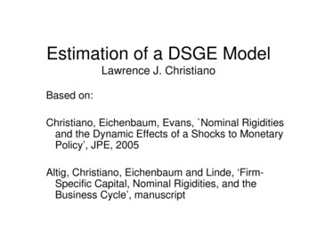
Evidence from Midrigan, ‘Menu Costs, Multi-Product Firms, and Aggregate Fluctuations’Lot’s ofsmallchangesHistogramsHitoff log(Pl (Pt/Pt-1),) conditionalditil on pricei adjustment,dj tt ffor ttwo ddatat setstpooled across all goods/stores/months in sample.

Households: Sequence of Events Technology shock realized. Decisions: Consumption, Capital accumulation, CapitalUtilization. Insurance markets on wage-setting open. Wage rate set. Monetary policy shock realized.realized Household allocates beginning of period cash betweendeposits at financial intermediary and cash to be used inconsumption transactions.

Dynamic Response of Consumption toMonetary Policy Shock In Estimated Impulse Responses:– Real Interest Rate FallsR t / t 1– Consumption Rises in Hump-Shape Pattern:ct

Consumption ‘Puzzle’ Intertemporal First Order Condition:‘Standard’ PreferencesMUc,tct 1 Rt / t 1 c t MUc,t 11 With Standard Preferences:ccData!tt

One Resolution to Consumption Puzzle Concave Consumption Response Displays:– Rising Consumption (problem)– FallingF lli SlopeSloff ConsumptionCtiHabit parameter Habit Persistence in ConsumptionU c log c b c 1 – Marginal Utility Function of Slope of Consumption– Hump-Shape Consumption Response Not a Puzzle Econometric Estimation Strategy Given the Option, b 0

Dynamic Response of Investment toMonetary Policy Shock In Estimated Impulse Responses:– Investment Rises in Hump-Shaped Pattern:It

Investment ‘Puzzle’ Rate of Return on CapitalRktMPkt 1 Pk′,t 1 1 ,Pk′,tPk′,t consumption price of installed capitalMPkt marginal product of capital 0,1 0 1 depreciationdepreciation rate.rate Rough ‘Arbitrage’ Condition:Rt Rk.t t 1 Positive Money Shock Drives Real Rate:kRt Problem: Burst of Investment!

One Solution to Investment Puzzle AdjustmentAdj tt CostsC t ini IInvestmenttt– Standard Model (Lucas-Prescott)– Problem:k′ 1 k F I I.k Hump-Shape Response Creates AnticipatedCapital GainsP k ′ ,t 1t 1IP k ′,t 1Optimal Under StandardSpecificationtIData!t

One Solution to InvestmentPPuzzle l CostCost-of-Changeof Change Adjustment Costs:k′ 1 k F II 1 I ThiThis DDoes PProducedaHHump-ShapeShInvestment Response– Other Evidence Favors This Specification– Empirical: Matsuyama, Smets-Wouters.– Theoretical: MatsuyamaMatsuyama, David Lucca

Financial Frictions In the standard model, household does thesaving needed to produce capital, and thehousehold is also the one that puts thecapital to work (i.e., rents it out and decidesits utilization rate). In practice, the saving decision and theoperation of capital is done by differentpeople. These different people may have aconflict of interest. Conflict of interest leads to ‘frictions’ (a lossof resources)

Bernanke-Gertler-Gilchristmodel Source of friction:– People who provide funds and people who putfunds to work are different people– When funds are put to work, idiosyncratic thingshappen that are known only to the people puttingthe funds to work.– Savers and borrowers can’t just share the output,because borrowers have an incentive tomisreport earningsearnings.

Entrepreneur off Type ω,Where Eω 1.BankHouseholdsL d FundsLendF dto BanksR t 1 t MP k,t 1 P k ′,t 1 1 P k ′,tFinancial friction

Wage Decisions Households supply differentiated laborlabor. Standard Calvo set up as in Erceg,Henderson and Levin and CEECEE.

Parameter estimatesTABLE 2: ESTIMATED PARAMETER VALUES 1 fModel wBenchmark 1. 35 . 75 0.17 0.06 abS ′′ . 32 0. 06 0. 80 4. 85 0. 77 0.32 0.18 0.04 2.15 0.27 PParameterstare surprisinglyi i l consistenti t t withith estimatesti treported in JPE (2005) based on studying only monetarypolicy shocks Note slope of Phillips curve is fairly large, but standard error islarge too!– At point estimates: p 0. 58,1 2. 38 quarters1 p Other parameters ‘reasonable’: estimation results really wantsticky wages!

Parameters of exogenous shocks:TABLE 3:3 ESTIMATED PARAMETER VALUES 2 M M z z xzczpcz x c pc Benchmark Model 0. 10 0. 31 . 91 0. 05 0. 36 3. 68 2. 49 0. 24 0. 17 0. 91 0. 10 0. 63 0.12 0.10 0.03 0.02 0.22 1.55 1.22 0.52 0.06 0.07 0.57 Neutral technology shock, z ,is highlypersistentpersistent. 0.65

Implications of the Estimated Model forthe Distribution of Production AcrossFirms

Summary We constructed a dynamic GE model of cyclical fluctuations. Given assumptionspsatisfied byy our model, we identified dynamicyresponse of key US economic aggregates to 3 shocks– Monetary Policy Shocks– Neutral Technology Shocks– Capital Embodied Technology Shocks These shocks account for substantial cyclical variation in output. Estimated GE model does a good job of accounting for responsefunctions (However, Misses on Inflation Response to Neutral Shock) Our point estimates suggest slope of Phillips curve steep, so there isno micro-macro price puzzle. However, large standard error.

Summary Summary Calvo Sticky Prices and Wages SeemsLike Good Reduced Form– What is the Underlying Structure?– Is it information frictions?

Agency Employment Agency Employment unemployment Agency Employment Agency. Firm Sector Final Good, Competitive Fims Intermediate Good Producer 1 Intermediate Good . Insurance markets on wage-setting open. Wage rate set. Monetary policy shock realizedMonetary policy shock realized.