Transcription
Argia M. Sbordone, Andrea Tambalotti, Krishna Rao, and Kieran WalshPolicy Analysis Using DSGEModels: An Introduction Dynamic stochastic general equilibriummodels are playing an important role in theformulation and communication of monetarypolicy at many of the world’s central banks. These models, which emphasize thedependence of current choices on expectedfuture outcomes, have moved from academiccircles to the policymaking community—butthey are not well known to the general public. This study adds to the understanding of theDSGE framework by using a small-scalemodel to show how to address specificmonetary policy questions; the authorsfocus on the causes of the sudden pickupin inflation in the first half of 2004. An important lesson derived from the exerciseis that the management of expectations canbe a more effective tool for stabilizing inflationthan actual movements in the policy rate;this result is consistent with the increasingfocus on central bankers’ pronouncementsof their future actions.Argia M. Sbordone is an assistant vice president and Andrea Tambalotti asenior economist at the Federal Reserve Bank of New York; Krishna Rao isa graduate student at Stanford University; Kieran Walsh is a graduate studentat Yale University.Correspondence: argia.sbordone@ny.frb.org, andrea.tambalotti@ny.frb.org1. IntroductionIn recent years, there has been a significant evolution inthe formulation and communication of monetary policyat a number of central banks around the world. Many ofthese banks now present their economic outlook and policystrategies to the public in a more formal way, a processaccompanied by the introduction of modern analytical toolsand advanced econometric methods in forecasting and policysimulations. Official publications by central banks thatformally adopt a monetary policy strategy of inflationtargeting—such as the Inflation Report issued by the Bankof England and the monetary policy reports issued by theRiksbank and Norges Bank—have progressively introducedinto the policy process the language and methodologiesdeveloped in the modern dynamic macroeconomic literature.1The development of medium-scale DSGE (dynamicstochastic general equilibrium) models has played a key rolein this process.2 These models are built on microeconomicfoundations and emphasize agents’ intertemporal choice.The dependence of current choices on future uncertain1The Bank of England has published a quarterly Inflation Report since 1993.The report sets out the detailed economic analysis and inflation projections onwhich the Bank’s Monetary Policy Committee bases its interest rate decisions.The Riksbank and Norges Bank each publish monetary policy reports threetimes a year. These reports contain forecasts for the economy and anassessment of the interest rate outlook for the medium term.2A simple exposition of this class of models can be found in Galí and Gertler(2007). Woodford (2003) provides an exhaustive textbook treatment.The authors thank Ariel Zetlin-Jones for his contribution to the early stagesof this work. The views expressed are those of the authors and do notnecessarily reflect the position of the Federal Reserve Bank of New Yorkor the Federal Reserve System.FRBNY Economic Policy Review / October 201023
outcomes makes the models dynamic and assigns a centralrole to agents’ expectations in the determination of currentmacroeconomic outcomes. In addition, the models’ generalequilibrium nature captures the interaction between policyactions and agents’ behavior. Furthermore, a more detailedspecification of the stochastic shocks that give rise to economicfluctuations allows one to trace more clearly the shocks’transmission to the economy.The use of DSGE models as a potential tool for policyanalysis has contributed to their diffusion from academic topolicymaking circles. However, the models remain less wellknown to the general public. To broaden the understanding ofthese models, this article offers a simple illustration of how anestimated model in this class can be used to answer specificmonetary policy questions. To that end, we introduce thestructure of DSGE models by presenting a simple model,meant to flesh out their distinctive features. Before proceedingto a formal description of the optimization problems solved byfirms and consumers, we use a simple diagram to illustratethe interactions among the main agents in the economy. Withthe theoretical structure in place, we discuss the features of theestimated model and the extent to which it approximates thevolatility and comovement of economic time series. We alsodiscuss important outcomes of the estimation—namely, theThis article offers a simple illustration ofhow an estimated [DSGE] model . . . canbe used to answer specific monetarypolicy questions.possibility of recovering the structural shocks that driveeconomic fluctuations as well as the historical behavior ofvariables that are relevant for policy but are not directlyobservable. We conclude by applying the DSGE tool to studythe role of monetary policy in a recent episode of an increase ininflation. The lesson we emphasize is that, while they are a verystylized representation of the real economy, DSGE modelsprovide a disciplined way of thinking about the economicoutlook and its interaction with policy.3We work with a small model in order to make thetransmission mechanism of monetary policy, whose basiccontours our model shares with most DSGE specifications,as transparent as possible. Therefore, the model focuses onthe behavior of only three major macroeconomic variables:inflation, GDP growth, and the short-term interest rate.3Adolfson et al. (2007) offer a more extended illustration of how DSGE modelscan be used to address questions that policymakers confront in practice. Erceg,Guerrieri, and Gust (2006) illustrate policy simulations with an open-economyDSGE model.24Policy Analysis Using DSGE Models: An IntroductionHowever, the basic framework that we present could easilybe enriched to provide more details on the structure of theeconomy. In fact, a key advantage of DSGE models is that theyshare core assumptions on the behavior of households andfirms, which makes them easily scalable to include details thatare relevant to address the question at hand. Indeed, severalA key advantage of DSGE models is thatthey share core assumptions on thebehavior of households and firms, whichmakes them easily scalable to includedetails that are relevant to address thequestion at hand.extensions of the basic framework presented here have beendeveloped in the literature, including the introduction of wagestickiness and frictions in the capital accumulation process(see the popular model of Smets and Wouters [2007]) and atreatment of wage bargaining and labor market search (Gertler,Sala, and Trigari 2008).4 Recently, the 2008 financial crisis hashighlighted one key area where DSGE models must develop:the inclusion of a more sophisticated financial intermediationsector. There is a large body of work under way to modelfinancial frictions within the baseline DSGE framework—workthat is very promising for the study of financial intermediationas a source and conduit of shocks as well as for its implicationsfor monetary policy. However, this last generation of modelshas not yet been subjected to extensive empirical analysis.Our study is organized as follows. Section 2 describes thegeneral structure of our model while Section 3 illustrates itsconstruction from microeconomic foundations. Section 4briefly describes our approach to estimation and presents someof the model’s empirical properties. In Section 5, we use themodel to analyze the inflationary episode of the first half of2004. Section 6 concludes.2. DSGE Models and TheirBasic StructureDynamic stochastic general equilibrium models used for policyanalysis share a fairly simple structure, built around threeinterrelated blocks: a demand block, a supply block, and a4Some of these larger DSGE models inform policy analysis at central banksaround the world: Smets and Wouters (2007) of the European Central Bank;Edge, Kiley, and Laforte (2008) of the Federal Reserve System; and Adolfsonet al. (2008) of the Riksbank.
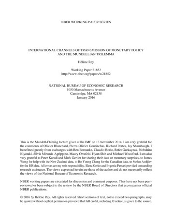
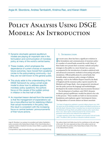
The Basic Structure of DSGE ModelsMark-upshocksDemandshocksY f YY(Y e, i - π ee,.)DemandProductivityshocksπ f π(π e,Y,.)SupplyY e,π eExpectationsi f i(π π *,Y,.)Monetary policyPolicyshocksmonetary policy equation. Formally, the equations that definethese blocks derive from microfoundations: explicitassumptions about the behavior of the main economic actorsin the economy—households, firms, and the government.These agents interact in markets that clear every period, whichleads to the “general equilibrium” feature of the models.Section 3 presents the microfoundations of a simple DSGEmodel and derives the equations that define its equilibrium.But first, we begin by introducing the basic componentscommon to most DSGE models with the aid of a diagram.In the diagram, the three interrelated blocks are depicted asrectangles. The demand block determines real activity Y asa function of the ex ante real interest rate—the nominal rateeminus expected inflation i – —and of expectations aboutefuture real activity Y . This block captures the idea that, whenreal interest rates are temporarily high, people and firms wouldrather save than consume or invest. At the same time, peopleare willing to spend more when future prospects are promisinge( Y is high), regardless of the level of interest rates.The line connecting the demand block to the supply blockshows that the level of activity Y emerging from the demandblock is a key input in the determination of inflation ,etogether with expectations of future inflation . Inprosperous times, when the level of activity is high, firms mustincrease wages to induce employees to work longer hours.Higher wages increase marginal costs, putting pressure onprices and generating inflation. Moreover, the higher inflationis expected to be in the future, the higher is this increase inprices, thus contributing to a rise in inflation today.The determination of output and inflation from thedemand and supply blocks feeds into the monetary policyblock, as indicated by the dashed lines. The equation in thatblock describes how the central bank sets the nominal interestrate, usually as a function of inflation and real activity. Thisreflects the tendency of central banks to raise the short-terminterest rate when the economy is overheating as well as wheninflation rises and to lower it in the presence of economic slack.By adjusting the nominal interest rate, monetary policy in turnaffects real activity and through it inflation, as represented bythe line flowing from the monetary policy block to the demandblock and then to the supply block. The policy rule thereforecloses the circle, giving us a complete model of the relationshipbetween three key endogenous variables: output Y , inflation , and the nominal interest rate i .While this brief description appears static, one of thefundamental features of DSGE models is the dynamicinteraction between the blocks—hence, the “dynamic” aspectof the DSGE label—in the sense that expectations about thefuture are a crucial determinant of today’s outcomes. Theseexpectations are pinned down by the same mechanism thatgenerates outcomes today. Therefore, output and inflationOne of the fundamental features ofDSGE models is the dynamic interactionbetween the [three interrelated] blocks—hence, the “dynamic” aspect of the DSGElabel—in the sense that expectationsabout the future are a crucial determinantof today’s outcomes.tomorrow, and thus their expectations as of today, depend onmonetary policy tomorrow in the same way as they do today—of course, taking into account what will happen from thenon into the infinite future.The diagram highlights the role of expectations and thedynamic connections between the blocks that they create.The influence of expectations on the economy is represented bythe arrows, which flow from monetary policy to the demandand then the supply block, where output and inflation aredetermined. This is to emphasize that the conduct of monetarypolicy has a large influence on the formation of expectations.In fact, in DSGE models, expectations are the main channelthrough which policy affects the economy, a feature that isconsistent with the close attention paid by financial marketsand the public to the pronouncements of central banks on theirlikely course of action.The last component of DSGE models captured in thediagram is their stochastic nature. Every period, randomexogenous events perturb the equilibrium conditions in eachblock, injecting uncertainty in the evolution of the economyFRBNY Economic Policy Review / October 201025
and thus generating economic fluctuations. Without theseshocks, the economy would evolve along a perfectly predictablepath, with neither booms nor recessions. We represent theseshocks as triangles, with arrows pointing toward theequilibrium conditions on which they directly impinge. Markup and productivity shocks, for example, affect the pricing andproduction decisions of firms that underlie the supply block,while demand shocks capture changes in the willingness ofhouseholds to purchase the goods produced by those firms.3. Microfoundations of a SimpleDSGE ModelWe present the microfoundations of a small DSGE model thatis simple enough to fit closely into the stylized structureoutlined in our diagram. Our objective is to describe the basiccomponents of DSGE models from a more formal perspective,using the mathematical language of economists, but avoidingunnecessary technical details. Despite its simplicity, our modelis rich enough to provide a satisfactory empirical account of theevolution of output, inflation, and the nominal interest rate inthe United States in the last twenty years, as we discuss in thenext section.Given the constraints we impose on this treatment for thesake of simplicity, our model lacks many features that arestandard in the DSGE models that central banks typically use.For example, we ignore the process of capital accumulation,Despite its simplicity, our model is richenough to provide a satisfactory empiricalaccount of the evolution of output,inflation, and the nominal interest rate inthe United States in the last twenty years.which would add another dimension—investment decisionsby firms—to the economy’s demand block. Nor do we attemptto model the labor market in detail: for example, we make nodistinction between the number of hours worked by eachemployee and the number of people at work, an issue that ishard to overlook in a period with unemployment close to10 percent. Finally, we exclude any impediment to the smoothfunctioning of financial markets and assume that the centralbank can perfectly control the short-term interest rate—theonly relevant rate of return in the economy. The 2008 financialcrisis has proved that this set of assumptions can fail miserably26Policy Analysis Using DSGE Models: An Introductionin some circumstances and has highlighted the need for amore nuanced view of financial markets within the currentgeneration of DSGE models, as we observe in our introduction.3.1. The Model EconomyOur model economy is populated by four classes of agents:a representative household, a representative final-goodproducing firm (f-firm), a continuum of intermediate firms(i-firms) indexed by i 0 1 , and a monetary authority. Thehousehold consumes the final good and works for the i-firms.Each of these firms is a monopolist in the production of aparticular intermediate good i , for which it is thus able toOur model economy is populated byfour classes of agents: a representativehousehold, a representative final-goodproducing firm, . . . a continuum ofintermediate firms, . . . and a monetaryauthority.set the price. The f-firm packages the differentiated goodsproduced by the i-firms and sells the product to households ina competitive market. The monetary authority sets the nominalinterest rate.The remainder of this section describes the problem facedby each economic agent, shows the corresponding optimization conditions, and interprets the shocks that perturb theseconditions. These optimization conditions result in dynamicrelationships among macroeconomic variables that define thethree model blocks described above. Together with marketclearing conditions, these relationships completely characterizethe equilibrium behavior of the model economy.3.2. Households and the AggregateDemand BlockAt the core of the demand side of virtually all DSGE modelsis a negative relationship between the real interest rate anddesired spending. In our simple model, the only source ofspending is consumption. Therefore, the negative relationshipbetween the interest rate and demand emerges from theconsumption decision of households.
We model this decision as stemming from the optimalchoice of a very large representative household—the entireU.S. population—which maximizes its expected discountedlifetime utility, looking forward from an arbitrary date t 0 s Et bt s log Ct sMax000 s 0 s 0 Bt s Ct s Ht s i To find the solution to the optimal problem above, we formthe Lagrangian s bt 0 s log Ct s – Ct s – 1 L Et000 s 0 000– Cti 0 1 10 s–1 0 – v Ht0 sBPt C t -----t B t – 1 Rt– t i di subject to the sequence of budget constraints– Bt0 s Pt0 s–10 s–Ct1 0 Wt0 s0 s i di Bt0 s–1 0 sRt , i Ht s i di 0 s0with first-order conditions1 0 wt i Ht i di ,for t t 0 t 0 1 , , and given Bt – 1. The members of this0household, we call them “Americans,” like consumption, Ct ,but dislike the number of hours they spend at work, Ht , toan extent described by the convex function . The utilityflow from consumption depends on current as well as pastconsumption, with a coefficient . As a result of this “habit,”consumers are unhappy if their current consumption is low,but also if it falls much below the level of their consumption inthe recent past. To afford consumption, Americans work acertain amount of hours Ht i in each of the i-firms, where theyearn an hourly nominal wage Wt i which they take as givenwhen deciding how much to work.5 With the income thusearned, they can purchase the final good at price Pt or save byaccumulating one-period discount government bonds Bt ,whose gross rate of return between t and t 1 is Rt .From the perspective of time t , the household discountsutility in period t 1 by a time-varying factor bt 1 bt , wherebt 1 bt is an exogenous stochastic process. Changes in bt 1 btrepresent shocks to the household’s impatience. When bt 1increases relative to bt , for example, the household cares moreabout the future and thus wishes to save more and consumeless today, everything else equal. In this respect, bt 1 bt acts asa traditional demand shock, which affects desired consumptionand saving exogenously. A persistent increase in bt 1 bt is oneway of interpreting the current macroeconomic situation in theUnited States, in which households have curtailed theirconsumption—partly to build their savings. Of course, inreality there are many complex reasons behind this observedchange in behavior, and an increase in people’s concern aboutthe future is surely one of them. For simplicity, the modelfocuses on this one reason exclusively.51 0– v HtIn equilibrium, the wage—and thus the number of hours worked—will settleat the level at which the supply of labor by the household equals the demand oflabor by firms. This labor demand in turn is determined by the need of firmsto hire enough workers to satisfy the demand for their products, as we describein the next section.(3.1a)(3.1b) L------: t Et t 1 R t Bt bt 1 bt L 1-------- : -----t P -------------------------- .– Et -------------------------C Ct bt tCt – Ct – 1t 1 – Ctfor t t 0 t 0 1 , and(3.2) Ht i L--------------- : --------------------- Wt i Ht i t btfor t t 0 t 0 1 , and i 0 1 , together with thesequence of budget constraints.These conditions yield a fully state-contingent plan for thehousehold’s choice variables—how much to work, consume,and save in the form of bonds—looking forward from theplanning date t 0 and into the foreseeable future. At any pointin time, the household is obviously uncertain about the wayin which this future will unfold. However, we assume that thehousehold is aware of the kind of random external events, orshocks, that might affect its decisions and, crucially, that itknows the probability with which these shocks might occur.Therefore, the household can form expectations about futureoutcomes, which are one of the inputs in its current choices.We assume that these expectations are rational, meaning thatthey are based on the same knowledge of the economy and ofthe shocks that buffet it as that of the economist constructingthe model. We use the notation Et X t s to denoteexpectations formed at time t of any future variable X t s ,as in equations 3.1, for example. The optimal plan, then,is a series of instructions on how to behave in response to therealization of each shock, given expectations about the future,rather than a one-time decision on exactly how much towork, consume, and save on each future date.Together, the optimality conditions in equations 3.1establish the negative relationship between the interest rate anddesired consumption that defines the demand side of themodel. The nature of this relationship is more transparent inthe special case of no habit in consumption ( 0 ), when weFRBNY Economic Policy Review / October 201027
can combine the two equations to obtain(3.3)Rt bt 1 11- .- ----------- ----------------------- E t ------------bt C t 1 Pt 1 PtCtAccording to this so-called Euler equation, desiredconsumption decreases when the (gross) real interest rateRt ------------------- increases, when expected future consumption Pt 1 Pt decreases, and when households become more patient( bt 1 rises).A log-linear approximation of the Euler equation (3.3),after some manipulation, gives(3.4)yt Et yt 1 – i t – Et t 1 – t ,where t log Pt Pt – 1 is the quarterly inflation rate, i t log Rtis the continuously compounded nominal interest rate, t Et log bt 1 bt is a transformation of the demand shock,and y t log Yt is the logarithm of total output. In thisexpression, we can substitute consumption of the final good Ctwith its output Yt because in our model consumption is theonly source of demand for the final good. Therefore, marketclearing implies Yt Ct .In this framework, equation 3.4 is similar to a traditional ISequation, since it describes the relationship between aggregateactivity y t and the ex ante real interest rate i t – Et t 1 , whichmust hold for the final-good market to clear. Unlike atraditional IS relationship, though, this equation is dynamicand forward looking, as it involves current and future expectedvariables. In particular, it establishes a link between currentoutput and the entire future expected path of real interest rates,as we see by solving the equation forward (3.5)yt – Et it s – t s 1 – t s .s 0Through this channel, expectations of future monetary policydirectly affect current economic conditions. In fact, thisequation shows that future interest rates are just as importantto determine today’s output as the current level of the shortterm rate, as we describe in our discussion of the role of policyexpectations.In our full model, the Euler equation is somewhat morecomplicated than in equation 3.4 because of the consumptionhabit ( 0), which is a source of richer, and more realistic,output dynamics in response to changes in the interest rate.Nevertheless, these more intricate dynamics do not change thequalitative nature of the relationship between real rates anddemand.The third first-order condition of the householdoptimization problem, equation 3.2, represents the laborsupply decision. It says that Americans are willing to workmore hours in firms that pay a higher wage and at times when28Policy Analysis Using DSGE Models: An Introductionwages are higher, at least for differences in wages modestenough to have no significant effect on their income.6 Largewage changes, in fact, would trigger an income effect andlead the now richer workers to curtail their labor supply.Mathematically, workers with higher income could affordmore consumption, which would lead to a drop in the marginalutility t and thus to a decrease in labor supply at any givenwage level.We can think of the labor supply schedule (equation 3.2)as a relationship determining the wage that firms must payto induce Americans to work a certain number of hours.In prosperous times, when demand is high and firms areproducing much, firms require their labor force to work longhours and they must correspondingly pay higher hourly wages.This is an important consideration in the production andpricing decisions of firms, as we discuss in the next section.3.3. Firms and the Aggregate Supply BlockThe supply block of a DSGE model describes how firms settheir prices as a function of the level of demand they face. Recallthat in prosperous times, demand is high and firms must paytheir workers higher wages. As a result, their costs increase asdo their prices. In the aggregate, this generates a positiverelationship between inflation and real activity.In terms of microfoundations, establishing this relationshiprequires some work, since firms must have some monopolypower to set prices. This is why our production structureincludes a set of monopolistic i-firms, which set prices, as wellas an f-firm, which simply aggregates the output of the i-firminto the final consumption good. Because all the pricing actionoccurs within the i-firms, we focus on their problem and omitthat of the f-firm.Intermediate firm i hires Ht i units of labor of type i ona competitive market to produce Yt i units of intermediategood i with the technology(3.6)Yt i At Ht i ,where At represents the overall efficiency of the productionprocess. We assume that At follows an exogenous stochasticprocess, whose random fluctuations over time capture theunexpected changes in productivity often experienced bymodern economies—for example, the productivity boom inthe mid-1990s that followed the mass adoption of informationtechnology. We call this process an aggregate productivity shock,since it is common to all firms.Labor supply is upward sloping because is an increasing function, as isconvex. In other words, people dislike working an extra hour more intenselywhen they are already working a lot rather than when they are working little.6
The market for intermediate goods is monopolisticallycompetitive, as in Dixit and Stiglitz (1977), so firms set pricessubject to the requirement that they satisfy the demand fortheir good. This demand comes from the f-firm and takesthe formPt i – t(3.7),Yt i Yt ----------Pt where Pt i is the price of good i and t is the elasticity ofdemand. When the relative price of good i increases, itsdemand falls relative to aggregate demand by an amountthat depends on t .Moreover, we assume that firms change their prices onlyinfrequently. The fact that firms do not adjust pricescontinuously, but leave them unchanged in some cases for longperiods of time, should be familiar from everyday experienceand is well established in the economic literature (for example,Bils and Klenow [2004]; Nakamura and Steinsson [2008]). Tomodel this fact, we follow Calvo (1983) and assume that inevery period only a fraction 1 – of firms is free to reset itsprice while the remaining fraction maintains its old price.7The subset of firms that are able to set an optimal price at t ,call it t 0 1 , maximize the discounted stream of expectedfuture profits, taking into account that s periods from nowsthere is a probability that they will be forced to retain theprice chosen today. The objective function of each of thesefirms is therefores s t s---------------- Pt i Yt s i – Wt s i Ht s i Max E t tPPt i s 0for all i t , subject to the production function 3.6 and to theadditional constraint that they must satisfy the demand fortheir product at every point in timePt i – t s(3.8),Yt s i Yt s ---------- Pt s for s 0 , 1, , . Profits, which are given by total revenueat the price chosen today, Pt i Yt s i minus total costssWt s i Ht s i , are discounted by the multiplier t s t ,sometimes called a stochastic discount factor, which translatesdollar profits in the future into a current dollar value.The first-order condition of this optimization problem is t s – 1Wt s i s- 0, t s Yt s Pt sPt i – t s -----------------(3.9) E tAt s s 0for all i t , where Pt i denotes the optimal price chosen byfirm i , Wt s i At s is the firm’s nominal marginal cost at time t s –1t s , and t s ---------------- is its desired mark-up—the mark-up t sIn our estimated model in Section 5, we actually assume that the fractionof firms that cannot choose their price freely can in fact adjust it in part to catchup with recent inflation. This assumption improves the model’s ability to fit thedata on inflation, but it would complicate our presentation of the model’smicrofoundations without altering its basic message.it would charge if prices were flexible. As rational monopolists,optimizing firms set their price as a mark-up over theirmarginal cost. However, this relationship holds in expectedpresent discounted value, rather than every period, since asprice chosen at time t will still be in effect with prob
v ----- -, - - - - ----- - ----- ------ ----- - - ----- - , ----- .