Transcription
ClickHereJOURNAL OF GEOPHYSICAL RESEARCH, VOL. 114, D02102, doi:10.1029/2008JD010485, 2009forFullArticleData mining for evolution of association rules for droughts and floodsin India using climate inputsC. T. Dhanya1 and D. Nagesh Kumar1Received 23 May 2008; revised 20 October 2008; accepted 10 November 2008; published 22 January 2009.[1] An accurate prediction of extreme rainfall events can significantly aid in policymaking and also in designing an effective risk management system. Frequent occurrencesof droughts and floods in the past have severely affected the Indian economy, whichdepends primarily on agriculture. Data mining is a powerful new technology which helpsin extracting hidden predictive information (future trends and behaviors) from largedatabases and thus allowing decision makers to make proactive knowledge-drivendecisions. In this study, a data-mining algorithm making use of the concepts of minimaloccurrences with constraints and time lags is used to discover association rulesbetween extreme rainfall events and climatic indices. The algorithm considers only theextreme events as the target episodes (consequents) by separating these from the normalepisodes, which are quite frequent, and finds the time-lagged relationships with theclimatic indices, which are treated as the antecedents. Association rules are generated forall the five homogenous regions of India and also for All India by making use of thedata from 1960 to 1982. The analysis of the rules shows that strong relationships existbetween the climatic indices chosen, i.e., Darwin sea level pressure, North AtlanticOscillation, Nino 3.4 and sea surface temperature values, and the extreme rainfall events.Validation of the rules using data for the period 1983–2005 clearly shows that most of therules are repeating, and for some rules, even if they are not exactly the same, thecombinations of the indices mentioned in these rules are the same during validationperiod, with slight variations in the classes taken by the indices.Citation: Dhanya, C. T., and D. Nagesh Kumar (2009), Data mining for evolution of association rules for droughts and floods inIndia using climate inputs, J. Geophys. Res., 114, D02102, doi:10.1029/2008JD010485.1. Introduction[2] Asian monsoon greatly influences most of the tropicsand subtropics of the eastern hemisphere and more than60% of the earth’s population [Webster et al., 1998]. Whilethe failure of the monsoon brings famine, an excess orstrong monsoon will result in devastating floods, particularly if they are unanticipated. An accurate prediction ofthese two extremes (drought and flood) can help decisionmakers to improve planning to mitigate the adverse impactsof monsoon variability and to take advantage of beneficialconditions [Webster et al., 1998]. From the early 1900s,various climatic and oceanic parameters had been used aspredictors for monsoon rainfall prediction. Thus, if theassociation of the extremes with the climatic and oceanicparameters can be revealed, this can be used for designingan effective risk management system for facing the extremes.[3] India receives major portion of its annual rainfallduring the south west monsoon season (June – September).Even a small variation in this seasonal rainfall can have an1Department of Civil Engineering, Indian Institute of Science,Bangalore, India.Copyright 2009 by the American Geophysical Union.0148-0227/09/2008JD010485 09.00adverse impact on Indian economy. As per the IndianMeteorological Department (IMD), an annual rainfall eventis considered a drought (flood) if it is less (greater) than onestandard deviation from the long-term average annualrainfall. According to this definition, in the past 50 years,India has experienced around 10 droughts and 9 floods withhighest intensity of drought and flood in 1972 and 1959respectively. Two multiyear droughts also occurred in the1960s and 1980s. The frequency and intensity of drought ismuch more than of the flood.[4] Recent studies in the variation of the Gross DomesticProduct (GDP) and the monsoon [Gadgil and Gadgil, 2006]have showed that the impact of severe droughts is about 2 to5% of the GDP throughout. This indicates the need fortaking proactive steps to address the impacts of both therainfall extremes which in turn demand for an accurateprediction of the occurrence and nonoccurrence of theextremes. It is also shown that the impact of deficit rainfall(drought) on GDP is larger than that of surplus rainfall(flood).[5] Studies on the prediction of Indian Summer MonsoonRainfall (ISMR) have used various empirical and physical(atmospheric and coupled) models. A brief history of thesestudies and the models and predictors used is shown inTable 1. A comparative study between empirical andphysical models [Goddard et al., 2001] has shown thatD021021 of 15
D02102DHANYA AND KUMAR: DROUGHT AND FLOOD ASSOCIATION RULESD02102Table 1. Models Used for Prediction of Indian Summer Monsoon s UsedDarwin sea level pressure,latitudinal position of 500-mbridge along 75 EArabian sea SSTDarwin sea level pressure,latitudinal position of500-mb ridge along 75 E,May surface resultantwind speedNorthern Australia-IndonesiaSST, Darwin pressureIndian Ocean SSTQuasi biennial oscillation,sea surface temperatureanomalies over differentNino regionsDarwin sea level pressure tendency,Nino 3.4, NAO, quasi biennialoscillation, western Pacific regionSST, eastern Indian Ocean regionSST, Arabian Sea region SST,Eurasian surface temperature,and Indian surface temperatureEquatorial east Indian Ocean seasurface temperatureIndian summer monsoon rainfallArabian Sea SST, Eurasian snow cover,northwest Europe temperature,Nino 3 SST anomaly (previous year),south Indian Ocean SST index,East Asia pressure, Northern Hemisphere50-hPa wind pattern, Europepressure gradient, south IndianOcean 850-hPa zonal wind,Nino 3.4 SST tendency,North Indian Ocean-NorthPacific Ocean 850-hPa zonalwind difference, North AtlanticOcean SSTNino 3.4 and Equatorial zonal Wind INdex(EQWIN)First stage predictors:North Atlantic SST anomaly,equatorial SE Indian Oceananomaly, East Asia surfacepressure anomaly, Europe landsurface air temperature anomaly,northwest Europe surfacepressure anomaly tendency,Equatorial Pacific Warm Water Volume(WWV) anomalySecond stage predictors: firstthree first-stage predictors,Nino 3.4 SST anomaly tendency,North Atlantic surface pressureanomaly, North Central Pacificzonal wind anomaly at 850 hPaArabian Sea SST and centralequatorial Indian Ocean SSTNino 3.4 and EQWINNino 3.4 and EQWINTechniqueReferenceLinear regression modelShukla and Mooley [1987]Nonlinear gravity modelNeural networkDube et al. [1990]Navone and Ceccatto [1994]Correlation analysisNicholls [1995]Linear regression modelCorrelation analysisClarke et al. [2000]Chattopadhyay and Bhatla [2002]Linear regression modelDelSole and Shukla [2002];DelSole and Shukla [2006]Correlation analysisReddy and Salvekar [2003]Neural network Linear regressionPower regression modelIyengar and Raghu Kanth [2004]Rajeevan et al. [2004]Bayesian dynamic linear modelsMaity and Nagesh Kumar [2006]Ensemble multiple linear regressionmodel and projection pursuitregression modelRajeevan et al. [2006]Simple regression modelSadhuram [2006]Correlation and phase plane analysisSemiparametric, copula-based approachGadgil et al. [2007]Maity and Nagesh Kumar [2008]empirical models continue to outperform physical models inprediction of ISMR, as most of the physical models areunable to simulate accurately the interannual variability ofISMR. However the skill of any of these models in predicting the extremes is not satisfactory [Gadgil et al., 2005].None of these models could successfully predict the droughtsof 2002 and 2004. One of the reasons for the inability ofthese models to capture the relationship of the extremes withthe predictors may be due to the infrequent occurrence of theextremes. Assuming the rainfall distribution as a normal fre-2 of 15
D02102DHANYA AND KUMAR: DROUGHT AND FLOOD ASSOCIATION RULESquency curve, the occurrence of either drought or floodcovers only 16% of the time (since only 16% of the distribution area is less than the mean 1 standard deviation).[6] In this study, a time series data-mining algorithmis used to generate the association rules between oceanicand atmospheric parameters and rainfall extremes. In thisattempt, attention is given to find the relationship betweenonly the extremes and the predictors, without consideringthe normal rainfall which is quite frequent. By using such adata-mining algorithm in this context, one of the advantagesis that there is no need to have a prior idea about thecorrelation and causal relationships between the variables.Unlike the empirical methods, this method takes intoaccount the interrelationships between the predictor variables very well. The exact values of the model parameterssuch as coefficients in a regression model or weights in aneural network are of little importance in this approach.Thus the objective here is to unearth all the frequent patterns(episodes) of the predictors that precede the extreme episodes of rainfall using a time series data-mining algorithm.2. Time Series Data Mining[7] Data mining can be defined as a process in whichspecific algorithms are used for extracting some newnontrivial information from large databases. Data-miningtechniques are widely applied in business activities and alsoin scientific and engineering scenarios. Various data-miningtechniques can be broadly classified into two types [Hanand Kamber, 2006]: descriptive data mining, in which thedata in the database are characterized according to theirgeneral properties and predictive data mining, in whichpredictions are made by performing inference from thecurrent data. Frequent patterns and association rules, clustering and deviation detection come under the first categorywhile regression and classification come under the secondone. Almost all the studies done so far on rainfall extremesare based on the predictive data-mining techniques. Asmentioned earlier, these studies were unable to successfullypredict the infrequent extreme episodes. Hence, in thisstudy, a descriptive data-mining technique is used to captureespecially the infrequent extreme episodes.[8] Temporal data mining is concerned with data miningof large sequential sets (ordered data with respect to someindex). Time series is a popular class of sequential data inwhich records are indexed by time. The possible objectivesin the case of temporal data mining can be grouped asfollows: (1) prediction, (2) classification, (3) clustering,(4) search and retrieval, and (5) pattern discovery [Hanand Kamber, 2006]. Among these, algorithms of patterninterest are of most recent origin. The word ‘‘pattern’’means a local structure in the data. The objective is tosimply unearth all patterns of interest. One common measure to assess the value of a pattern is the frequency of thepattern. A frequent pattern is one that occurs many times inthe data. The frequent patterns thus discovered can be usedto discover the causal rules.[9] A rule consists of a left-hand side proposition (antecedent) and a right hand side proposition (consequent). Therule states that when the antecedent occurs (is true), then theconsequent also occurs (is true). Rule based approaches areD02102often used to ascertain the relationships within the data set.For example, association rules determine the rules thatindicate whether or how much the values of an attributedepend on the values of the other attributes in the data set.These are used to capture correlations between differentattributes in the data. In such cases, the conditional probability of the occurrence of the consequent given the antecedent is referred to as the confidence of the rule. Forexample, if a pattern ‘‘B follows A’’ occurs n1 times and thepattern ‘‘C follows B follows A’’ occurs n2 times, then thetemporal association rule ‘‘whenever B follows A, C willalso follow’’ has a confidence of (n2/n1). The value of a ruleis usually measured in terms of its confidence.[10] There are two popular frameworks for frequentpattern discovery namely sequential patterns and episodes.In the sequential patterns framework, a collection of sequences are given and the task is to discover the order ofsequences of the items (i.e., sequential patterns) that occursin sufficiently good number of those sequences. In thefrequent episodes framework, the data are given in a singlelong sequence and the task is to unearth temporal patterns(called episodes) that occur sufficiently often along thatsequence. Frequent episodes framework is used in thepresent study, since one does not know in prior all thesequences to be searched in the time series as is required insequential patterns framework. Also, concern is to extractthe temporal patterns of the climatic indices and extremeevents which can be done by applying frequent episodesframework. Several algorithms were formulated [Mannila etal., 1997] for the discovery of frequent episodes within onesequence.2.1. Framework of Frequent Episode Discovery2.1.1. Event Sequence[11] The data, referred to here as an event sequence, aredenoted by h(E1, t1), (E2, t2),. . .i where Ei takes values froma finite set of event types e, and ti is an integer denoting thetime stamp of the ith event. The sequence is ordered withrespect to the time stamps so that, ti ti 1 for all i 1, 2,. . .The following is a sample event sequence with six eventtypes A, B, C, D, E and F in it:[12] Any event sequence can be expressed as a tripleelement (s, TB, TD) where s is the time-ordered sequence ofevents from beginning to end, TB is the beginning time andTD is the ending time.The above sample event sequencecan be expressed as S (s, 9, 43) where s h(B, 10), (C, 11),(A, 12), (F, 13), (A, 15), . . . (C, 42)i.2.1.2. Episode[13] An episode a is defined by a triple element (Va, a,ga), where Va is a collection of nodes, a is a partial orderon Va and ga: Va ! e is a map that associates each node inthe episode with an event type. Thus an episode is acombination of events with a time-specified order. Whenthere is a fixed order among the event types of an episode, itis called a serial episode and when there is no order at all,the episode is called a parallel episode.3 of 15
D02102DHANYA AND KUMAR: DROUGHT AND FLOOD ASSOCIATION RULES[14] An episode is said to occur in an event sequence ifthere exist events in the sequence occurring in exactly thesame order as that prescribed in the episode, within a giventime bound. For example, in the above sample eventsequence, the events (A, 19), (B, 21) and (C, 22) constitutean occurrence of a 3-node serial episode (A ! B ! C)while the events (A, 12), (B, 10) and (C, 11) do not, because for this serial episode to occur, A must occur beforeB and C.2.1.3. Window[15] Now, to find all frequent episodes from a class ofepisodes, the user has to define how close is close enoughby defining a time window width within which the episodesshould appear. For an episode to be interesting, the events inan episode must occur close to each other in time span. Awindow can be defined as a slice of an event sequence andthen the event is considered as a sequence of partiallyoverlapping windows. A window on an event sequence (s,Ts, Te) can also be expressed as a triple element w (w, ts,te)., where ts Te, te Ts and w consists of those event pairsfrom s where ts ti te. The time span te ts is called thewidth of the window w.[16] Consider the example of event sequence givenabove. Two windows of width 5 are shown. The firstwindow starting at time 10 is shown in solid line, followedby a second window shown in dashed line. First window canbe represented as (h(B, 10), (C, 11), (A, 12), (F, 13)i, 10, 15).Here the event (A, 15) occurred at the ending time is notincluded in the sequence. Similarly, the second window canbe represented as (h(C, 11), (A, 12), (F, 13), (A, 15)i, 11, 16).[17] For a sequence S with a given window width ‘‘win’’,the total number of windows possible is given by W(s, win) Te Ts win. This is because the first and last windowsextend outside the sequence, such that the first windowcontains only the first time stamp of the sequence and thelast window contains only the last time stamp. Hence an eventclose to either end of a sequence is observed in equally manywindows to an event in the middle of the sequence. For thesequence given above, totally there are 39 partially overlapping windows with first window (F, 5, 10) and lastwindow (F, 43, 48).[18] The frequency of an episode is defined as the numberof windows in which the episode occurs divided by the totalnumber of windows in the data set. For the 3-node serialepisode (A ! B ! C), there are only two occurrences i.e.,in windows (h(F, 18), (A, 19), (B, 21), (C, 22), 18, 23) and(h(A, 19), (B, 21), (C, 22), (E, 23)i, 19, 24). Thus thefrequency of the episode is (2/39) 100 5.13%. Now,given an event sequence, a window width and a frequencythreshold, the task is to discover all frequent episodes in theevent sequence.[19] Once the frequent episodes are known, it is possibleto generate rules that describe temporal correlations between events. However, there can be other ways to defineepisode frequency.2.1.4. MINEPI Algorithm[20] One such alternative proposed by Mannila et al.[1997] is MINEPI algorithm and is based on counting whatare known as minimal occurrences of episodes. A minimaloccurrence of an episode is defined as a window (orcontiguous slice) of the input sequence in which the episodeoccurs, subject to the condition that no proper subwindowD02102of this window contains an occurrence of the episode. Thealgorithm for counting minimal occurrences trades spaceefficiency for time efficiency as compared to the windowsbased counting algorithm. In addition, since the algorithmlocates and directly counts occurrences (as against countingthe number of windows in which episodes occur), itfacilitates the discovery of patterns with extra constraints(such as being able to discover rules of the form ‘‘if A and Boccur within 10 seconds of one another, C follows withinanother 20 seconds’’).[21] Minimal occurrences of episodes with their timeintervals are identified in the following way. For a givenepisode a and an event sequence S, the minimal occurrenceof a in S is the interval [ts, te], if (1) a occurs in the windoww (w, ts, te) on S, and if (2) a does not occur in any propersubwindow on w. A window w0 (w0, t0s, t0e) will be a propersubwindow of w if ts t0s, t0e te, and width(w0) width(w). The set of minimal occurrences of an episode ain a given event sequence is denoted by mo(a) {[ts, te)j[ts,te)} . For the example sequence given above, the serialepisode a B ! C has four minimal occurrences i.e.,mo(a) {[10,11), [21,22), [32,36), [38,42)}.[22] The concept of frequency of episodes explained inthe previous section is not very useful in the case ofminimal occurrences as there is no fixed window size andalso a window may contain several minimal occurrences ofan episode. Therefore Mannila et al. [1997] used theconcept of support instead of frequency. The support ofan episode a in a given event sequence S is jmo(a)j. Anepisode a is frequent if jmo(a)juser defined minimumsupport threshold.2.1.5. MOWCATL Algorithm[23] The above approach was modified to handle separateantecedent and consequent constraints and maximum window widths and also the time lags between the antecedentand consequent to find natural delays embedded within theepisodal relationships by Harms and Deogun [2004] inMinimal Occurrences With Constraints And Time Lags(MOWCATL) algorithm. Although MINEPI and MOWCATL both use the concept of minimal occurrences to findthe episodal relationships, MOWCATL has some additionalmechanisms like (1) allowing a time lag between theantecedent and consequent of a discovered rule, and (2)working with episodes from across multiple sequences[Harms et al., 2002]. Episodal rules are found out wherethe antecedent episode occurs within a given maximumwindow width wina, the consequent episode occurs within agiven maximum window width winc, and the start of theconsequent follows the start of the antecedent within a givenmaximum time lag. This algorithm allows to find rules ofthe form: ‘‘if A and B occur within 3 months, then within 2months they will be followed by C and D occurring togetherwithin 4 months’’.[24] This algorithm first goes through the data sequenceand stores the occurrences of all single events for theantecedent and consequent separately. The algorithm onlylooks for the target episodes specified by the user. So itprunes the episodes that do not meet the user specifiedminimum support threshold. Then two event episodes aregenerated by pairing up the single events so that the pairs ofevents occur within the prescribed window width and theoccurrences of these two event episodes in the data se-4 of 15
D02102DHANYA AND KUMAR: DROUGHT AND FLOOD ASSOCIATION RULESD02102Figure 1. Homogenous monsoon regions of India, as defined by the Indian Institute of TropicalMeteorology.quence are recorded. This is repeated until there are no moreevents to be paired up. The process repeats for three events,four events and so on until there are no episodes left to becombined that meet the minimum threshold. The frequentepisodes for antecedent and consequent sequences are foundindependently. These frequent episodes are combined toform an episodal rule.[25] An episodal rule is that in which an antecedentepisode occurs within a given window width, a consequentepisode occurs within a given window width and the start ofthe consequent follows the start of the antecedent within auser specified time lag. For example, let episode X is of theevents A and B, and episode Y is of the events C and D.Also the user specified antecedent window width is 3months, consequent window width is 2 months and thetime lag is 3 months. Then the rule generated would indicatethat if A and B occur within 3 months, then within 3 monthsthey will be followed by C and D occurring together within2 months. The support of the rule is the number of times therule occurs in the data sequence. The confidence of the ruleis the conditional probability that the consequent occurs,given the antecedent occurs. For the rule ‘‘X is followed byY’’, the confidence is the ratio of the Support[X and Y] andSupport[X]. Here X is a serial antecedent episode (A ! B)and Y is a serial consequent episode (C ! D).[26] The support and confidence are the two measuresused for measuring the value of the rule. The values of theseare set high to prune the association rules. Even after settingthe threshold of these measures high, there will be anadequate number of rules, making the user’s task of ruleselection difficult. The user needs some quantifying measures to select the most valuable rules in addition to thesupport and confidence measures. Several interestingness orgoodness measures are used to compare and select betterrules from the ones that are generated [Bayardo andAgarwal, 1999; Das et al., 1998; Harms et al., 2002]. InMOWCATL algorithm, J measure is used for rule ranking[Smyth and Goodman, 1991]. The J measure is given by2J ð x; yÞ ¼ pð xÞ4pð yjxÞ log½ pð yjxÞ pð yÞ þ35½1 pð yjxÞ logf½1 pð yjxÞ ½1 pð yÞ gð1Þwhere p(x), p(y) and p(yjx) are the probabilities ofoccurrence of x, y and y given x respectively in the datasequence. The first term in the J measure is a bias towardrules which occur more frequently. The second term i.e., theterm inside the square brackets is well known as crossentropy, namely the information gained in going from the5 of 15
DHANYA AND KUMAR: DROUGHT AND FLOOD ASSOCIATION RULESD02102D02102Table 2. Threshold Values Used for the Categorization of Monthly Rainfall (mm) for Various Regions and Also for All IndiaaRegionExtremeDroughtNorthwestWest centralCentral northeastNortheastPeninsularAll India 150 1100 1200 2200 1000 1200Severe Drought15011001200220010001200 XXXXXX 50014501600270012001500Moderate Drought50014501600270012001500 XXXXXX 85019002000310014501800Normal Rainfall850 X 15501900 X 26002000 X 28503100 X 39001450 X 19001800 X 2400Moderate Flood155026002850390019002400 XXXXXX 190030003300430021002700Severe Flood190030003300430021002700 XXXXXX 0023502900aRainfall in millimeters.prior probability p(y) to a posterior probability p(yjx) [Daset al., 1998]. Compared to other measures which directlydepend on the probabilities [Piatetsky-Shapiro, 1991],thereby assigning less weight to the rarer events, J measureis better suited to rarer events since it uses a log scale(information based). As shown by Smyth and Goodman[1991], J measure has the unique properties as a ruleinformation measure and is a special case of Shannon’smutual information.[27] The J values range from 0 to 1. The higher the Jvalue the better it is. However, since drought and flood areso infrequent, the J values are so small that all values greaterthan 0.025 are to be considered.[28] MOWCATL algorithm is used in the present studyfor extracting rules between extreme episodes and climaticindices, since this algorithm can be used for multiplesequences and also this will capture by itself the lagbetween the occurrences of climatic indices and rainfallevents.3. Data Used for the Study[29] The time series data sets used in this study are of themonthly values for the period 1960 to 2005 and are definedas follows.[30] 1. Summer monsoonal rainfall (June to September)for All India and also for the five homogeneous regions (asdefined by Indian Institute of Tropical Meteorology), for theperiod 1960 to 2005 (http://www.tropmet.res.in).[ 31 ] 2. Darwin sea level pressure (DSLP), s).[32] 3. Nino 3.4, east central tropical Pacific sea surfacetemperature (SST), 170 E – 120 W, 5 S – 5 N ndices).[33] 4. North Atlantic Oscillation (NAO), normalized sealevel pressure difference between Gibraltor and southwestIceland (http://www.cru.uea.ac.uk/cru/data/nao.htm).[34] 5. 1 1 degree grid SST data over the region 40 E–120 E, 25 S – 25 N (ICOADS, ).4. Association Rules for Extremes[35] The data-mining algorithm is applied to find theassociation rules of the extreme rainfall episodes with theclimatic indices and thus to find the spatial and temporalpatterns of extreme episodes throughout the country. Thegeographical locations of the homogenous regions: northwest, central northeast, northeast, west central and peninsular are shown in Figure 1.Figure 2. Summer monsoon rainfall for the northwest region for the period 1960– 2005 indicating thethreshold values to classify droughts and floods.6 of 15
D02102DHANYA AND KUMAR: DROUGHT AND FLOOD ASSOCIATION RULESD02102Figure 3. Summer monsoon rainfall for the west central region for the period 1960 – 2005 indicating thethreshold values to classify droughts and floods.4.1. Selection of Consequent Episodes[36] In order to identify the extreme episodes, the rainfallfor All India and also for the five homogenous regions isdivided into seven categories. The threshold values aredetermined by identifying the values at 1.5, 1 and 0.5standard deviations from the average. Threshold valuescalculated for each region are given in Table 2. The sevenclasses thus identified are named as: moderate drought,severe drought, extreme drought, normal rainfall, moderateflood, severe flood and extreme flood. Although from ahydrologic point of view, greater than normal rainfall cannotbe called as a flood, for a better classification, in thiscontext, greater than normal rainfall are divided into 3categories and are called as moderate, severe and extremeflood. Same is applicable for the classification of less thannormal rainfall also. For example, while considering thenortheast region, a rainfall value of less than or equal to2200 mm/month is under the category of extreme droughtalthough it will not result to any ‘‘real’’ drought.[37] For application of the algorithm, only the extremeepisodes (moderate drought, severe drought, extremedrought, moderate flood, severe flood and extreme flood)Figure 4. Summer monsoon rainfall for the central northeast region for the period 1960– 2005indicating the threshold values to classify droughts and floods.7 of 15
D02102DHANYA AND KUMAR: DROUGHT AND FLOOD ASSOCIATION RULESD02102Figure 5. Summer monsoon rainfall for the northeast region for the period 1960 –2005 indicating thethreshold values to classify droughts and floods.are specified as the target episodes. The summer monsoonrainfall (JJAS) time series of each region and also of AllIndia for the period 1960 – 2005, indicating the thresholdvalues are shown in Figures 2 –7.4.2. Selection of Antecedent Episodes[38] 1 1 degree grid SST data over the region 40 E–120 E, 25 S – 25 N are averaged to a 5 5 degree griddata, thus reducing to 127 grids (excluding the land arearegions). Among these, the most influencing grids areselected by plotting the correlation contour plots considering different lags for each region. Grids used for correlationanalysis (numbered 1 to 127) are shown in Figure 8. Themaximum correlation of SST with the summer monsoon isachieved at lag 7 for all the regions. The correlation contoursfor northwest region for lag 7 is shown in Figure 9. TheFigure 6. Summer monsoon rainfall for the peninsular region for the period 1960– 2005 indicating thethreshold values to classify droughts and floods.8 of 15
D02102DHANYA AND KUMAR: DROUGHT AND FLOOD ASSOCIATION RULESD02102Figure 7. Summer monsoon rainfall for All India for the period 1960 – 2005 indicating the thresholdvalues to classify droughts and floods.variatio
study, a descriptive data-mining technique is used to capture especially the infrequent extreme episodes. [8] Temporal data mining is concerned with data mining of large sequential sets (ordered data with respect to some index). Time series is a popular class of sequential data in which records are indexed by time. The possible objectives in .