Transcription
Journal of Machine Learning Research 17 (2016) 1-30Submitted 4/15; Revised 5/16; Published 8/16Dual Controlfor Approximate Bayesian Reinforcement LearningEdgar D. stitute for Intelligent SystemsSpemannstraße 3872076 Tübingen, GermanyPhilipp stitute for Intelligent SystemsSpemannstraße 3872076 Tübingen, GermanyEditor: Manfred OpperAbstractControl of non-episodic, finite-horizon dynamical systems with uncertain dynamics poses atough and elementary case of the exploration-exploitation trade-off. Bayesian reinforcementlearning, reasoning about the effect of actions and future observations, offers a principledsolution, but is intractable. We review, then extend an old approximate approach fromcontrol theory—where the problem is known as dual control —in the context of modernregression methods, specifically generalized linear regression. Experiments on simulatedsystems show that this framework offers a useful approximation to the intractable aspectsof Bayesian RL, producing structured exploration strategies that differ from standard RLapproaches. We provide simple examples for the use of this framework in (approximate)Gaussian process regression and feedforward neural networks for the control of exploration.Keywords:inferencereinforcement learning, control, Gaussian processes, filtering, Bayesian1. IntroductionThe exploration-exploitation trade-off is a central problem of learning in interactive settings,where the learner’s actions influence future observations. In episodic settings, where thecontrol problem is re-instantiated repeatedly with unchanged dynamics, comparably simplenotions of exploration can succeed. E.g., assigning an exploration bonus to uncertain options(Macready and Wolpert, 1998; Audibert et al., 2009) or acting optimally under one samplefrom the current probabilistic model of the environment (Thompson sampling, see Thompson,1933; Chapelle and Li, 2011), can perform well (Dearden et al., 1999; Kolter and Ng, 2009;Srinivas et al., 2010). Such approaches, however, do not model the effect of actions on futurebeliefs, which limits the potential for the balancing of exploration and exploitation. Thisissue is most drastic in the non-episodic case, the control of a single, ongoing trial. Here, thecontroller cannot hope to be returned to known states, and exploration must be carefullycontrolled to avoid disaster. 2016 Edgar D. Klenske and Philipp Hennig.
Klenske and HennigA principled solution to this problem is offered by Bayesian reinforcement learning (Duff,2002; Poupart et al., 2006; Hennig, 2011): A probabilistic belief over the dynamics andcost of the environment can be used not just to simulate and plan trajectories, but also toreason about changes to the belief from future observations, and their influence on futuredecisions. An elegant formulation is to combine the physical state with the parametersof the probabilistic model into an augmented dynamical description, then aim to controlthis system. Due to the inference, the augmented system invariably has strongly nonlineardynamics, causing prohibitive computational cost—even for finite state spaces and discretetime (Poupart et al., 2006), all the more for continuous space and time (Hennig, 2011).The idea of augmenting the physical state with model parameters was noted early, andtermed dual control, by Feldbaum (1960–1961). It seems both conceptual and—by thestandards of the time—computational complexity hindered its application. An exception is astrand of several works by Meier, Bar-Shalom, and Tse (Tse et al., 1973; Tse and Bar-Shalom,1973; Bar-Shalom and Tse, 1976; Bar-Shalom, 1981). These authors developed techniquesfor limiting the computational cost of dual control that, from a modern perspective, canbe seen as a form of approximate inference for Bayesian reinforcement learning. While theBayesian reinforcement learning community is certainly aware of their work (Duff, 2002;Hennig, 2011), it has not found widespread attention. The first purpose of this paper is tocast their dual control algorithm as an approximate inference technique for Bayesian RL inparametric Gaussian (general least-squares) regression. We then extend the framework withideas from contemporary machine learning. Specifically, we explain how it can in principlebe formulated non-parametrically in a Gaussian process context, and then investigate simple,practical finite-dimensional approximations to this result. We also give a simple, small-scaleexample for the use of this algorithm for dual control if the environment model is constructedwith a feedforward neural network rather than a Gaussian process.2. Model and NotationThroughout, we consider discrete-time, finite-horizon dynamic systems (POMDPs) of formxk 1 fk (xk , uk ) ξkyk Cxk γk(state dynamics)(observation model).At time k {0, . . . , T }, xk Rn is the state, ξk N (0, Q) is a Gaussian disturbance. Thecontrol input (continuous action) is denoted uk ; for simplicity we will assume scalar uk Rthroughout. Measurements yk Rd are observations of xk , corrupted by Gaussian noiseγk N (0, R). The generative model thus reads p(xk 1 xk , uk ) N (xk 1 ; fk (xk , uk ), Q)and p(yk xk ) N (yk ; Cxk , R), with a linear map C Rd n . Trajectories are vectorsx [x0 , . . . , xT ], and analogously for u, y. We will occasionally use the subset notationy i j [yi , . . . , yj ]. We further assume that dynamics fk are not known, but can be describedup to Gaussian uncertainty by a general linear model with nonlinear features φ Rn Rmand uncertain matrices Ak , Bk .xk 1 Ak φ(xk ) Bk uk ξk ,Ak Rn m ; Bk Rn 1 .(1)To simplify notation, we reshape the elements of Ak and Bk into a parameter vectorθk [vec(Ak ); vec(Bk )] R(m 1)n , and define the reshaping transformations A(θk ) θk Ak2
Dual Control for Approximate Bayesian Reinforcement Learningand B(θk ) θk Bk . At initialization, k 0, the belief over states and parameters isassumed to be Gaussianx̂0xxΣxx Σxθ0 ]) .p ([ 0 ]) N ([ 0 ] ; [ ] , [ 0θxθ0θ0Σ0 Σθθθ̂00(2)The control response Bk uk is linear, a common assumption for physical systems. Nonlinearmappings can be included in a generic form φ(xk , uk ), but complicate the following derivationsand raise issues of identifiability. For simplicity, we also assume that the dynamics do notchange through time: p(θk 1 θk ) δ(θk 1 θk ). This could be relaxed to an autoregressivemodel p(θk 1 θk ) N (θk 1 ; Dθk , Ξ), which would give additive terms in the derivationsbelow. Throughout, we assume a finite horizon with terminal time T and a quadratic costfunction in state and controlTT 1k 0k 0L(x, u) [ (xk rk ) Wk (xk rk ) u k Uk uk ] ,where r [r0 , . . . , rT ] is a target trajectory. Wk and Uk define state and control cost, theycan be time-varying. The goal, in line with the standard in both optimal control andreinforcement learning, is to find the control sequence u that, at each k, minimizes theexpected cost to the horizonJk (uk T 1 , p(xk )) Exk [(xk rk ) Wk (xk rk ) u k Uk uk Jk 1 (uk 1 T 1 , p(xk 1 )) p(xk )] ,(3)where past measurements y 1 k , controls u1 k 1 and prior information p(x0 ) are incorporatedinto the belief p(xk ), relative to which the expectation is calculated. Effectively, p(xk ) servesas a bounded rationality approximation to the true information state. Since the equationabove is recursive, the final element of the cost has to be defined differently, asJT (p(xT )) ExT [(xT rT ) WT (xT rT ) p(xT )](that is, without control input and future cost). The optimal control sequence minimizingthis cost will be denoted u , with associated cost Jk (p(xk )) min Exk [(xk rk ) Wk (xk rk ) u k Uk uk Jk 1(p(xk 1 )) p(xk )] .uk(4)This recursive formulation, if written out, amounts to alternating minimization and expectation steps. As uk influences xk 1 and yk 1 , it enters the latter expectation nonlinearly.Classic optimal control is the linear base case (φ(x) x) with known θ, where u can befound by dynamic programming (Bellman, 1961; Bertsekas, 2005).3. Bayesian RL and Dual ControlFeldbaum (1960–1961) coined the term dual control to describe the idea now also known asBayesian reinforcement learning in the machine learning community: While adaptive controlonly considers past observations, dual control also takes future observations into account.This is necessary because all other ways to deal with uncertain parameters have substantial3
Klenske and Hennigdrawbacks. Robust controllers, for example, sacrifice performance due to their conservativedesign; adaptive controllers based on certainty equivalence (where the uncertainty of theparameters is not taken into account but only their mean estimates) do not show exploration,so that all learning is purely passive. For most systems it is obvious that more excitationleads to better estimation, but also to worse control performance. Attempts at finding acompromise between exploration and exploitation are generally subsumed under the term“dual control” in the control literature. It can only be achieved by taking the future effect ofcurrent actions into account.It has been shown that optimal dual control is practically unsolvable for most cases (Aoki,1967), with a few examples where solutions were found for simple systems (e.g., Sternby,1976). Instead, a large number of approximate formulations of the dual control problem wereformulated in the decades since then. This includes the introduction of perturbation signals(e.g., Jacobs and Patchell, 1972), constrained optimization to limit the minimal controlsignal or the maximum variance, serial expansion of the loss function (e.g., Tse et al., 1973)or modifications of the loss function (e.g., Filatov and Unbehauen, 2004). A comprehensiveoverview of dual control methods is given by Wittenmark (1995). A historical side-effect ofthese numerous treatments is that the meaning of the term “dual control” has evolved overtime, and is now applied both to the fundamental concept of optimal exploration, and tomethods that only approximate this notion to varying degree. Our treatment below studiesone such class of practical methods that aim to approximate the true dual control solution.The central observation in Bayesian RL / dual control is that both the states x andthe parameters θ are subject to uncertainty. While part of this uncertainty is caused byrandomness, part by lack of knowledge, both can be captured in the same way by probabilitydistributions. States and parameters can thus be subsumed in an augmented state (Feldbaum,1960–1961; Duff, 2002; Poupart et al., 2006) zk (x k θk ) R(m 2)n . In this notation,the optimal exploration-exploitation trade-off—relative to the probabilistic priors definedabove—can be written compactly as optimal control of the augmented system with a newobservation model p(yk zk ) N (yk ; C̃zk , R) using C̃ [C 0] and a cost analogous toEq. (3).Unfortunately, the dynamics of this new system are nonlinear, even if the original physicalsystem is linear. This is because inference is always nonlinear and future states influencefuture parameter beliefs, and vice versa. A first problem, not unique to dual control, isthus that inference is not analytically tractable, even under the Gaussian assumptionsabove (Aoki, 1967). The standard remedy is to use approximations, most popularly thelinearization of the extended Kalman filter (e.g., Särkkä, 2013). This gives a sequence ofapproximate Gaussian likelihood terms. But even so, incorporating these Gaussian likelihoodterms into future dynamics is still intractable, because it involves expectations over rationalpolynomial functions, whose degree increases with the length of the prediction horizon. Thefollowing section provides an intuition for this complexity, but also the descriptive power ofthe augmented state space.As an aside, we note that several authors (Kappen, 2011; Hennig, 2011) have previouslypointed out another possible construction of an augmented state: incorporating not theactual value of the parameters θk in the state, but the parameters µk , Σk of a Gaussian beliefp(θk µk , Σk ) N (θk ; µk , Σk ) over them. The advantage of this is that, if the state xk isobserved without noise, these belief parameters follow stochastic differential equations—more4
Dual Control for Approximate Bayesian Reinforcement Learningprecisely, Σk follows an ordinary (deterministic) differential equation, while µk follows astochastic differential equation—and it can then be attempted to solve the control problemfor these differential equations more directly.While it can be a numerical advantage, this formulation of the augmented state also hassome drawbacks, which is why we have here decided not to adopt it: First, the simplicity ofthe directly formalizable SDE vanishes in the POMDP setting, i.e. if the state is not observedwithout noise. If the state observations are corrupted, the exact belief state is not a Gaussianprocess, so that the parameters µk and Σk have no natural meaning. Approximate methodscan be used to retain a Gaussian belief (and we will do so below), but the dynamics of µk ,Σk are then intertwined with the chosen approximation (i.e. changing the approximationchanges their dynamics), which causes additional complication. More generally speaking, itis not entirely natural to give differing treatment to the state xk and parameters θk : Bothstate and parameters should thus be treated within the same framework; this also allowsextending the framework to the case where also the parameters do follow an SDE.3.1 A Toy ProblemTo provide an intuition for sheer complexity of optimal dual control, consider the perhapssimplest possible example: the linear, scalar systemxk 1 axk buk ξk ,(5)with target rk 0 and noise-free observations (R 0). If a and b are known, the optimal ukto drive the current state xk to zero in one step can be trivially verified to beu k,oracle abxk.U b2Let now parameter b be uncertain, with current belief p(b) N (b; µk , σk2 ) at time k. Thenaı̈ve option of simply replacing the parameter with the current mean estimate is known ascertainty equivalence (CE) control in the dual control literature (e.g., Bar-Shalom and Tse,1974). The resulting control law isu k,ce aµk xk.U µ2kIt is used in many adaptive control settings in practice, but has substantial deficiencies: Ifthe uncertainty is large, the mean is not a good estimate, and the CE controller might applycompletely useless control signals. This often results in large overshoots at the beginning orafter parameter changes.A slightly more elaborate solution is to compute the expected cost Eb [x2k 1 U u2k µk , σk2 ]and then optimize for uk . This gives optimal feedback (OF) or “cautious” control (Dreyfus,1964)1 :aµk xku k,of .(6)U σk2 µ2k1. Dreyfus used the term “open loop optimal feedback” for his approach, a term that is misleading tomodern readers, because it is in fact a closed-loop algorithm.5
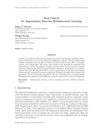
Klenske and HennigThis control law reduces control actions in cases of high parameter uncertainty. Thismitigates the main drawback of the CE controller, but leads to another problem: Sincethe OF controller decreases control with rising uncertainty, it can entirely prevent learning.Consider the posterior on b after observing xk 1 , which is a closed-form Gaussian (becauseuk is chosen by the controller and has no uncertainty):22) N (b; µk 1 , σk 1) N (b;p(b µk 1 , σk 1σk2 uk (buk ξk ) µk Qσk2 Q,)u2k σk2 Qu2k σk2 Q(7)(b shows up in the fully observed xk 1 axk buk ξk ). The dual effect here is that the2updated σk 1depends on uk . For large values of σk2 , according to (6), u k,of 0, and the2new uncertainty σk 1σk2 . The system thus will never learn or act, even for large xk . Thisis known as the “turn-off phenomenon” (Aoki, 1967; Bar-Shalom, 1981).However, the derivation for OF control above amounts to minimizing Eq. (3) for themyopic controller, where the horizon is only a single step long (T 1). Therefore, OF controlis indeed optimal for this case. By the optimality principle (e.g., Bertsekas, 2005), thismeans that Eq. (6) is the optimal solution for the last step of every controller. But since itdoes not show any form of exploration or “probing” (Bar-Shalom and Tse, 1976), a myopiccontroller is not enough to show the dual properties.In order to expose the dual features, the horizon has to be at least of length T 2. Sincethe optimal controller follows Bellman’s equation, the solution proceeds backwards. Thesolution for the second control action u1 is identical to the solution of the myopic controller(6); but after applying the first control action u0 , the belief over the unknown parameter bneeds an update according to Eq. (7), resulting inu 1 2 1 σ02 Qσ02 u0 (bu0 ξ0 ) µ0 Q σ02 u0 (bu0 ξ0 ) µ0 Q U 2 2 ()[ax1 ] . u0 σ0 Qu20 σ02 Qu20 σ02 Q (8)Inserting into Eq. (4) givesJ0 (x0 ) min Ex0 [W x20 U u20 min Ex1 [W x21 U u21 Ex2 [W x22 ]]]u1u0 min [W x20u0 U u20 Eξ0 ,b [W x21 U (u 1 )2 Eξ1 ,b [W (x1 bu 1 ξ1 )2 µ1 , σ1 ] µ0 , σ0 ]] .(9)Since u 1 from Eq. (8) is already a rational function of fourth order in b0 , and shows upquadratically in Eq. (9), the relevant expectations cannot be computed in closed form (Aoki,1967). For this simple case though, it is possible to compute the optimal dual control byperforming the expectation through sampling b, ξ0 , ξ1 from the prior. Fig. 1 shows suchsamples of L(u0 ) (in gray; one single sample highlighted in orange), and the empiricalexpectation J(u0 ) in dashed green. Each sample is a rational function of even leading order.In contrast to the CE cost, the dual cost is much narrower, leading to more cautious behaviorof the dual controller. The average dual cost has its minima not at zero, but to either sideof it, reflecting the optimal amount of exploration in this particular belief state.While it is not out of the question that the Monte Carlo solution can remain feasiblefor larger horizons, we are not aware of successful solutions for continuous state spaces6
4433costcostDual Control for Approximate Bayesian Reinforcement Learning210 121 0.50u00.50 11 0.50u00.51Figure 1: Left: Computing the T 2 dual cost for the simple system of Eq. (5). CostsL(u0 ) under optimal control on u1 for sampled parameter b (thin gray; one samplehighlighted, orange). Expected dual cost J(u0 ) under u 1 (dashed green). Theoptimal u 0 lies at the minimum of the dashed green line. Right: Comparisonof sampling (dashed green; thin gray: samples) to three approximations: CE(red) and CE with Bayesian exploration bonus (blue). The solid green line is theapproximate dual control constructed in Section 4. See also Sec. 6.1 for details.(however, see Poupart et al., 2006, for a sampling solution to Bayesian reinforcement learningin discrete spaces, including notes on the considerable computational complexity of thisapproach). The next section describes a tractable analytic approximation that does notinvolve samples.4. Approximate Dual Control for Linear SystemsIn 1973, Tse et al. (1973) constructed theory and an algorithm (Tse and Bar-Shalom, 1973)for approximate dual (AD) control, based on the series expansion of the cost-to-go. This isrelated to differential dynamic programming for the control of nonlinear dynamic systems(Mayne, 1966). It separates into three conceptual steps (described in Sec. 4.1–4.3), whichtogether yield what, from a contemporary perspective, amounts to a structured Gaussianapproximation to Bayesian RL: Find an optimal trajectory for the deterministic part of the system under the meanmodel: the nominal trajectory under certainty equivalent control. For linear systemsthis is easy (see below), for nonlinear ones it poses a nontrivial, but feasible nonlinearmodel predictive control problem (Allgöwer et al., 1999; Diehl et al., 2009). It yields anominal trajectory, relative to which the following step constructs a tractable quadraticexpansion. Around the nominal trajectory, construct a local quadratic expansion that approximatesthe effects of future observations. Because the expansion is quadratic, an optimalcontrol law relative to the deterministic system—the perturbation control —can beconstructed by dynamic programming. Plugging this perturbation control into theresidual dynamics of the approximate quadratic system gives an approximation for thecost-to-go. This step adds the cost of uncertainty to the deterministic control cost.7
Klenske and HennigComputeCE controlInitializepredict stateand covariancefor given uk Compute next valueuk for the searchno ComputeCE trajectoryand its covariancesMake newmeasurement Evaluatecost-to-goSimulate or runthe systemyessearch over?Apply thecontrolFigure 2: Flow-chart of the approximate dual control algorithm to show the overall structure.Adapted from Tse and Bar-Shalom (1973). The left cycle is the inner loop,performing the nonlinear optimization. In the current time step k, perform the prediction for an arbitrary control input uk(as opposed to the analytically computed control input for later steps). Optimize uknumerically by repeated computation of steps and at varying uk to minimize theapproximate cost.These three steps will be explained in detail in the subsequent sections. The interplaybetween the different parts of the algorithm is shown in Figure 2.The abstract introductory work Tse et al. (1973) is relatively general, but the explicitformulation in Tse and Bar-Shalom (1973) only applies to linear systems. Since both worksare difficult to parse for contemporary readers, the following sections thus first provide ashort review, before we extend to more modern concepts. In this section, we follow themore transparent case of a linear system from Tse and Bar-Shalom (1973), i.e. φ(x) xin Eq. (1). For the augmented state z, this still gives a nonlinear system, because θ and xinteract multiplicativelyzk 1 (xk 1A(θk ) 0B(θk )ξ) ()z () uk ( k ) f (zk , uk ).θk 10I k00(10)The parameters θ are assumed to be deterministic, but not known to the controller. Thisuncertainty is captured by the distribution p(θ) representing the lack of knowledge.4.1 Certainty Equivalent Control Gives a Nominal Reference TrajectoryThe certainty equivalent model is built on the assumption that the uncertain θ coincide withtheir most likely value, the mean θ̂ of p(θ), and that the system propagates deterministicallywithout noise. This means that the nominal parameters θ̄ are the current mean values θ̂,8
Dual Control for Approximate Bayesian Reinforcement Learningwhich decouples θ entirely from x in Eq. (10), and the optimal control for the finite horizonproblem can be computed by dynamic programming (DP) (Aoki, 1967), yielding an optimallinear control law 1ū j (B̄ K̄j 1 B̄ Uj ) B̄ [K̄j 1 Āx̄j p̄j 1 ] ,where we have momentarily simplified notation to Ā A(θ̄j ), B̄ B(θ̄j ), j, because the θ̄jare constant. The K̄j and p̄j for j k 1, . . . , T are defined and computed recursively asK̄j Ā (K̄j 1 K̄j 1 B̄ (B̄ K̄j 1 B̄ Uj ) 1p̄j Ā (p̄j 1 K̄j 1 B̄ (B̄ K̄j 1 B̄ Uj ) 1B̄ K̄j 1 ) Ā WjB̄ K̄j 1 ) p̄j 1 Wj rjK̄T WTp̄T WT rT ,where r is the reference trajectory to be followed. This CE controller gives the nominaltrajectory of inputs ūk T 1 and states x̄k T , from the current time k to the horizon T . The truefuture trajectory is subject to stochasticity and uncertainty, but the deterministic nominaltrajectory x̄, with its optimal control ū and associated nominal cost J k L(x̄k T , ū k T )provides a base, relative to which an approximation will be constructed.4.2 Quadratic Expansion Around the Nominal Defines Cost of UncertaintyThe central idea of AD control is to project the nonlinear objective Jk (uk T 1 , p(xk ))of Eq. (3) into a quadratic, by locally linearizing around the nominal trajectory x andmaintaining a joint Gaussian belief.To do so, we introduce small perturbations around nominal cost, states, and control: Jj Jj J j , zj zj z̄j , and uj uj ūj . These perturbations arise from both thestochasticity of the state and the parameter uncertainty. Note that a change in the stateresults in a change of the control signal, because the optimal control signal in each stepdepends on the state. Even though the origin of the uncertainties is different ( x arisesfrom stochasticity and θ from the lack of knowledge), both can be modeled in a jointprobability distribution.Approximate Gaussian filtering ensures that beliefs over z remain Gaussian:Σxx Σxθ x x̂jp( zj ) N [( j ) ; ( j ) , ( jθx)] . θj0ΣjΣθθjNote that shifting the mean to the nominal trajectory does not change the uncertainty.Note further that the expected perturbation in the parameters is nil. This is because theparameters are assumed to be deterministic and are not affected by any state or input.Calculating the Gaussian filtering updates is in principle not possible for future measurements, since it violates the causality principle (Glad and Ljung, 2000). Nonetheless, it ispossible to use the expected measurements to simulate the effects of the future measurementson the uncertainty, since these effects are deterministic. This is sometimes referred to aspreposterior analysis (Raiffa and Schlaifer, 1961).To second order around the nominal trajectory, the cost is approximated byJk (uk T 1 , p(xk )) J k Jk J k J k ,9
Klenske and Hennigwhere J k is the optimal cost for the nominal system and J k is the approximate additionalcost from the perturbation: TT 1 11 J k Exk T {(x̄j rj ) Wj xj x j Wj xj } {ū j Uj uj u j Uj uj } .22 j kj k (12)Although the uncertain parameters θ do not show up explicitly in the above equation, thisstep captures dual effects: The uncertainty of the trajectory x depends on θ via thedynamics. Higher uncertainty over θ at time j 1 causes higher predictive uncertainty over xj (for each j), and thus increases the expectation of the quadratic term x j Wj xj .Control that decreases uncertainty in θ can lower this approximate cost, modeling the benefitof exploration. For the same reason, Eq. (12) is in fact still not a quadratic function and hasno closed form solution. To make it tractable, Tse and Bar-Shalom (1973) make the ansatzthat all terms in the expectation of Eq. (12) can be written as gj p j zj 1/2 zj Kj zj .This amounts to applying dynamic programming on the perturbed system. Expectationsover the cost under Gaussian beliefs on z can then be computed analytically. Because all θ have zero mean, linear terms in these quantities vanish in the expectation. This allowsanalytic minimization of the approximate optimal cost for each time step11 J j (p(xj )) min {(xj rj ) Wj x̂j j x̂ j j Wj x̂j j u j U uj u j U uj uj221 tr [Wj Σxxj j ] E [ Jj 1 (y 1 j 1 ) p(xj )]} , (13) xj 12which is feasible given an explicit description of the Gaussian filtering update. It is importantto note that, assuming extended Kalman filtering, the update to the mean from expectedfuture observations yj 1 is nil. This is because we expect to see measurements consistentwith the current mean estimate. Nonetheless, the (co-)variance changes depending on thecontrol input uj , which is the dual effect.Following the dynamic programming equations for the perturbed problem, including theadditional cost from uncertainty, the resulting cost amounts to (Tse et al., 1973)1 J k (p(xk )) g̃k 1 p̃ k 1 ẑk ẑk K̃k 1 ẑk2 T 1 1 xx tr WT Σxx [WΣ (Σ Σ)K̃] j j jj 1 j 1 jj 1 j 1T T 2 j k (where we have neglected second-order effects of the dynamics). Recalling that ẑ 0 anddropping the constant part, the dual cost can be approximated to beJkd T 1 1 xxxx tr WT ΣT T [Wj Σj j (Σj 1 j Σj 1 j 1 )K̃j 1 ] 2 j k ( J k const)where the recursive equationxxK̃j à (K̃j 1 K̃j 1 B̃ (B Kj 1B Uj )10 1B̃ K̃j 1 ) à W̃jK̃T W̃T
Dual Control for Approximate Bayesian Reinforcement Learning is defined for the augmented system (10), with à zf , B̃ uf and W̃j blkdiag(Wj , 0). d The approximation to the overall cost is then Jk Jk , which is used in the subsequentoptimization procedure.4.3 Optimization of the Current Control Input Gives Approximate DualControlThe last step amounts to the outer loop of the overall algorithm. A gradient-free black-boxoptimization algorithm is used to find the minimum of the dual cost function. In every step,this algorithm proposes a control input uk for which the dual cost is evaluated.Depending on uk , approximate filtering is carried out to the horizon. The perturbationcontrol is plugged into Eq. (13) to give an analytic, recursive definition for K̃j , and anapproximation for the dual cost Jkd , as a function of the current control input uk .Nonlinear optimization—through repetitions of steps and for proposed locationsuk —then yields an approximation to the optimal dual control u k . Conceptually the simplestpart of the algorithm, this outer loop dominates computational cost, because for everylocation uk the whole machinery of and has to be evaluated.5. Extension to Contemporary Machine Learning ModelsThe preceding section reviewed the treatment of dual control in linear dynamical systemsfrom Tse and Bar-Shalom (1973). In this section, we extend the approach to inference on,and dual control of, the dynamics of nonlinear dynamical systems. This extension is guidedby the desire to use a number of popular, standard regression frameworks in machine learning:Parametric general least-squares regression, nonparametric Gaussian process regression, andfeedforward neural networks (including the base case of logistic regression).5.1 Parametric Nonlinear Syst
Bayesian reinforcement learning, reasoning about the e ect of actions and future observations, o ers a principled solution, but is intractable. We review, then extend an old approximate approach from . Bayesian reinforcement learning in the machine learning community: While adaptive control only considers past observations, dual control also .