Transcription
(IJACSA) International Journal of Advanced Computer Science and Applications,Vol. 13, No. 3, 2022Bayesian Hyperparameter Optimization andEnsemble Learning for Machine Learning Models onSoftware Effort EstimationRobert Marco1*, Sakinah Sharifah Syed Ahmad2, Sabrina Ahmad3Department of Informatics, Universitas Amikom Yogyakarta, Yogyakarta, Indonesia1Faculty of Information & Communication Technology, Universiti Teknikal Malaysia Melaka, Malaysia, Melaka, Malaysia2, 3Abstract—In recent decades, various software effortestimation (SEE) algorithms have been suggested. Unfortunately,generating high-precision accuracy is still a major challenge inthe context of SEE. The use of traditional techniques andparametric approaches is largely inaccurate because theyproduce biased and subjective accuracy. Meanwhile, none of themachine learning methods performed well. This study applies theAdaBoost ensemble learning method and random forest (RF), onthe other hand the Bayesian optimization method is applied todetermine the hyperparameters of this model. The PROMISErepository and the ISBSG dataset were used to build the SEEmodel. The developed model was comprehensively comparedwith four machine learning methods (classification andregression tree, k-nearest neighbor, multilayer perceptron, andsupport vector regression) under 3-fold cross validation (CV). Itcan be seen that the RF method based on AdaBoost ensemblelearning and bayesian optimization outperforms this approach.In addition, the AdaBoost-based model assigns a featureimportance rating, which makes it a promising tool in softwareeffort tlearning; random forest; software effort estimationI.ensembleINTRODUCTIONSoftware effort estimation (SEE) is a method of estimatingthe amount of time it will take to build a software system inperson-months or person-hours [1][2]. Uncertainty andimprecision characterize software effort estimationenvironments [3][4]. The topic of SEE, on the other hand, hasbeen characterized as a regression problem in general [5].Various SEE models in the literature still show considerableperformance deviations and are extremely dataset-dependent.SEE has previously been accomplished via expertjudgment, analogy, decomposition and recomposition, andparametric techniques [6]. Meanwhile, standard SEEmethodologies can produce erroneous estimates due to humanbias and subjectivity [7]. The Machine learning (ML)algorithm is very effective in modeling uncertainty as a betterdecision-making process [8]. However, no single learningmethod is ideal for all supervised learning tasks [9]. However,a single sophisticated algorithm may not be a consideration forbuilding current SEE models, as the performance of anymodel mainly depends on the characteristics of the data setused, such as data set size, outliers, categorical features, andmissing values.Several machine learning techniques have been widelyapplied in the SEE context which have been considered asnecessary steps, such as: Case-Based Reasoning (CBR),Artificial Neural Networks (ANN), Support VectorRegression (SVR) [10], while for other ML methods, such asRandom Forest (RF), Classification And Regression Tree(CART) and K-Nearest Neighbor (kNN), they are stillignored. RF is a powerful, easy-to-train ensemble learner withbig data [11]. RF is widely used in the data mining domainand has achieved good performance when dealing withregression and classification problems [12]; this method canovercome overfitting and is less affected by outliers [13]. Onthe other hand, RF improves prediction accuracy withoutsignificant computational improvement, and is not sensitive tomulticollinearity [14]. Some researchers have also applied RFto solve regression problems in the context of SEE, forexample [15][16][17]. Unfortunately, the RF model can onlybe extended horizontally because decision trees exist inparallel and these decision trees have equal weight in votingfor the final prediction even though some of these trees mayunderperform.The use of Ensemble learning combines several algorithmsthat process different hypotheses to make their predictionsperform well [18]. According to Lessmann et al. (2015), theensemble method is better than the single ML and otherstatistical method [19]. While, Kocaguneli et al. (2012), theproper use of the ensemble method can outperform theperformance of single learners on the ML model [20], as wellas being one of the best methods in increasing the accuracyand stability of the most influential estimation [21].Averaging, voting, and bagging are three common broadensemble approaches that have piqued the interest of machinelearning researchers. Meanwhile, developing ensemblemethods such as stacked generalization, AdaBoost algorithm,Gradient tree boosting have not been widely tried/ignored[22].Ren et al. (2016) investigated the use of ensembles inclassification and regression and the success of AdaBoostabout regression behaviour [23]. AdaBoost, as a popularboosting algorithm, combines weak estimators andimplements them on an improved version of the data with thehelp of weighted majority voting/hard voting [24]. However,AdaBoost may not offer high accuracy when the dataset isheavily contaminated with noise [25]. In contrast to, MartinDiaz et al. (2017), AdaBoost is also known to achieve a*Corresponding Author.419 P a g ewww.ijacsa.thesai.org
(IJACSA) International Journal of Advanced Computer Science and Applications,Vol. 13, No. 3, 2022significant reduction in bias as well [26], and low errorvariance [24]. Also, it is not easy to overfit during training[27].Unfortunately, the method will need to be fine-tuned to fitthe scenario at hand. Automatic hyperparameter adjustmentsaves time and effort when experimenting with differentmachine learning model configurations, improves algorithmaccuracy, and increases reproducibility. Hyperparametertuning is a well-known approach for achieving optimalperformance in machine learning models [28][29]. Severalother studies have shown that the accuracy dimension in SEEis strongly influenced by choice of information estimationusing parameter tuning techniques [30]. Because determiningthe best hyperparameter combination can improve the MLmodel's performance [28][31]. However, much of the workseems to implicitly assume that tuning the parameters will notsignificantly change the results [32]. In the worst case,improper parameter setting may lead to inferior performanceresults [33]. However, the default hyperparameter setting maynot produce consistent results depending on the data set used[34]. Based on the work by [35], there is still limited workinvestigating the impact of parameter setting for SEE methodsin improving prediction accuracy.Manual search, grid search, and random search are someof the most used hyperparameter optimization strategies [36].When the hyperparameter space is large, however, this methodis time consuming and impractical [6]. Manual searchnecessitates a higher level of professional knowledge, isdifficult to implement without prior experience, and takes time[37]. Meanwhile, grid search suffers from a dimensionalcurse, which means that as the number of hyperparameters setor the complexity of the search space and the range of valuesof the hyperparameters increases, the algorithm's efficiencydeclines dramatically [37]. Random search, on the other hand,is more effective in high-dimensional space [38], but thismethod is not reliable for training complex models [38].Despite the fact that this method provides automatic tuning, itcan acquire the optimization goal function's ideal globalimportance.Among other classic hyperparameter optimizationtechniques, Bayesian optimization is a very successfuloptimization algorithm for solving computationally expensivefunctions [39]. Bayesian hyperparameter optimizationtechnique to further promote generalization accuracy [40].Bayesian optimization is effective for problems with fewerhyperparameters and that are difficult to parallelize [6].Therefore, it promises to encourage the use of hyperparametertuning for further applications in SEE.Motivated by the benefits mentioned above, the AdaBoostRF-based method of ensemble learning was developed tocapture the relationships between features in an SEE context.To reduce time dependence and impracticality, Bayesianoptimization method is used to find suitable hyperparametermodels. The datasets in the PROMISE and ISBSG repositorieshave built the model in this paper. Based on literature review,there is still a limited use of the AdaBoost and RF ensemblelearning methods adopted to build the SEE model. Theremainder of this paper begins with related work, followed byexperimental design. Then, the results and discussioncontaining the comparison of models. At the end, discuss theconclusions and future work.II. RELATED WORKMeanwhile, the literature on offline learning does not havea supervised procedure for automatic parameter setting. In thecontext of offline SEE, the use of Classification andRegression Tree (CART) with the addition of more innovativefeatures can improve accuracy [28], the researchers used agrid search strategy to obtain optimal parameters for fivemachine learning techniques (KNN, Regression Trees (RT),MultilayerPerceptrons(MLP),Bagging RT,andBagging MLP) without used generating ensembles. Theresults revealed that while RT, Bagging RT, and KNN wereunaffected by tuning settings, MLP and Bagging MLP were.Minku (2019) Linear Regression in Logarithmic Scale(LogLR) results in a more stable prediction performance [41].Meanwhile, Minku and Yao (2013) investigated the RT,Bagging MLP, and Bagging RT techniques shown toperform well across several data sets. This suggests that thebest parameters to use with a machine learning approach maychange over time [35]. In the context of SEE, parametertuning in Support Vector Regression (SVR) is critical. A tabusearch has been proposed in particular to find the best SVRparameter tuning [42]. Elish (2013) conducted an empiricalstudy based on five machine learning approaches (KNN, SVR,MLP, Decision Tree (DT), and Radial Basis FunctionNetwork (RBFN)) that suggested a heterogeneous ensemble.Due to its irregular and unstable performance across thespecified data set, the single approach is unreliable.Furthermore, across all data sets, five machine learningapproaches were trained using the same configuration, but noexplanation for parameter tuning was supplied [43].Meanwhile, Villalobos-Arias and Quesada-López (2021)investigated CART, SVR, and ridge regression (RR) usingrandom search and grid search with six bio-inspiredalgorithms. The results demonstrate that the Flash Log SVRmodel is the most accurate in the most data sets, while theHyperband Log RR model is the most stable in the mostdatasets [44]. In particular, the stacked ensemble that offersthe best overall accuracy in this study takes the average of theestimated effort values generated by Bagging, RF, ABE,AdaBoost, Gradient boosting machine, and Ordinary leastsquares regression which are optimized using grid searchtechniques [25]. Meanwhile, Zakrani et al. (2018) used thegrid search (GS) method to improve SVR. The results showthat this approach can help improve the SVR technique'sperformance [45]. Stacking ensemble learning uses twohyperparameter tuning (Particle Swarm Optimization andGenetic Algorithms) while base learners (linear regression,MLP, RF, and Adaboost regressor). Experimental resultsreveal that the estimation accuracy is higher whenhyperparameters are set using PSO [6]. ROME (RapidOptimizing Methods for Estimation) is a configurationtechnique that uses sequential model-based optimization(SMO) to identify configuration settings for KNN, SVR, RF,and CART techniques. For both traditional and current tasks,ROME outperforms sophisticated approaches [46]. Theaccuracy and stability of SVR in SEE were tested to see how a420 P a g ewww.ijacsa.thesai.org
(IJACSA) International Journal of Advanced Computer Science and Applications,Vol. 13, No. 3, 2022random search hyperparameter tuning strategy affected them.According to the findings, the SVR set for random searchperformed similarly to the SVR set for grid search [47].Based on the findings of previous empirical investigationsin the context of SEE. This paper is different from previousresearch. The RF-based AdaBoost ensemble learning methodreinforced by the Bayesian optimization method was used tofind the appropriate hyperparameter model. Meanwhile, fourML techniques, such as: classification and regression tree(CART), k-nearest neighbor (k-NN), multilayer perceptron(MLP), and support vector regression (SVR) were used tocompare the performance results of the proposed SEE model.III. EXPERIMENTAL DESIGNThe data sets, ensemble learning, hyperparameter tuning,parameter setting ML, and evaluation measures utilized in thispaper are described in depth in this section.A. DatasetsThe most widely used datasets related to the SEE contextare the Repositories on PROMISE and ISBSG, among themost popular datasets. In 9 datasets from the public PROMISErepository (also known as SEACRAFT), as well as two subdatasets from the ISBSG10 and ISBSG18-IFPUG repositories.Table I lists the data set that was used in paper, includingthe number of projects, features, and categorical features. Thispaper uses eleven datasets (china, albrecht, maxwell, nasa93,cocomo81, kitchenham, kemerer, desharnais, and ISBSG10)and the preprocessing rules used in the study by [28][1], andthe UCP dataset according to the regulations [48]. Meanwhile,ISBSG18-IFPUG refers to research [44].B. Data PreprocessingThe Data Preprocessing approach in study was used toimprove prediction accuracy in the end. The DataPreprocessing technique is an effective option for effortestimation [50], is a crucial step in improving machinelearning performance [51]. According to Famili et al. (1997)the first step by removing features on the dataset that is notrelevant. Machine learning algorithms will perform better ifirrelevant features are removed [52]. Subsequent processingconverts information on categorical data into numeric. Ordinalcoding assigns a unique number code to each category [53],the advantage is that the dimensions of the problem space donot increase because each category is displayed as a singleinput [54]. Handling missing data by using kNNI (K-NearestNeighbor Imputation). This method proved to be efficient forestimating missing attribute values in various softwareengineering datasets [55]. In this study, data normalizationwas used as a scale of values 0 and 1. For all datasets, Mensahet al. (2018) discovered that the normalized Z-score [0,1]generated the best prediction accuracy when compared to boxcox and log transformation [56]. This research will utilize twosubsets at random: training (80%) and testing (20%) as apredicted evaluation of the training procedure.C. Random Forest AlgorithmFor regression purposes, the random forest is a set of tree)predictors (whererepresents theobserved input vector (covariate) of length with a randomvector associated with andis independent and identicallydistributed (iid) random vector. A regression setting where hasa numeric result, , but makes multiple points of contact withthe classification problem (categorical results). The observed(training) data are assumed to be taken independently of the)combined distribution () and consist of (()().For regression, the random forest prediction is theunweighted mean of the collection ̅ ( ) ( ) ().Forthe Law of Large Numbers ensures [57].̅ ( ))((())(1)The quantity on the right is the prediction (orgeneralization) error for a random forest, designated.Convergence in Eq. (1) implies that the random forest is notoverfit [57]. Determine the mean prediction error for the) as:individual tree ((())Assume that for all(), then yields:(2)the tree is unbiased, eg̅(3)Where ̅ is the weighted correlation between residuals() and() for independent.D. Adaboost Ensemble LearningAdaBoost is a popular variation of the original Boostingscheme [27]. AdaBoost is a robust ensemble approach forfitting a poor collection of learners to a enhanced data set. Thepredictions of the weak learner are merged using weightedsummation, to reproduce the final prediction [58]. TheAdaboost regressor is a high-accuracy ensemble learner that isused to tackle regression issues [59], Adaboost.R2, a modifiedversion of Adaboost.R, is used for regression [27].TABLE I.THE STUDY’S DATA SETDatasetSize 0421 P a g ewww.ijacsa.thesai.org
(IJACSA) International Journal of Advanced Computer Science and Applications,Vol. 13, No. 3, 2022Given, which is applied to the training set,seeks to improve the training data in each boosting iteration,using different weights. The first update iteration uses thesame weights and training data as before. The learner'salgorithm is then re-applied to the new weighted data, aftereach initial weight is updated. If the weights for the trainingdata that were predicted incorrectly in the previous phase areincreased, the weights for the training data that weresuccessfully predicted will be reduced. Finally, each weaklearner is compelled to concentrate on the sample that thepreceding one missed in the sequence [27]. In the following,Adaboost.R2 steps according to the rules [60][61]: Set the initial weight () to the training set. As the training set, define the original data's input (x)and target (y) variables. Install the regression model ( ) to the training set withthe notation. Get the predicted training target value:( )( ). Use the following equation to find the loss value for thei-th training sample ( ).[ ( )( ) ](4)Any function that is, can be used as the lossfunction ( ). Calculate the average loss ( ̅ ) for using thefollowing formula:̅ (5)When ̅ is smaller than 0.5, an appropriate forecast isproduced. If ̅ is more than 0.5, the weights should be updatedusing the equation below.(6)̅̅(7) To get the required loss function range, repeat steps 4-7.E. Bayesian with Gaussian Process Optimization of ModelHyperparametersBayesian optimization is a useful strategy for locating theby extremes of computationally expensive functions [39]. Inthis paper, Bayesian optimization is used in this research todiscover the maximum value at the sampling point for theunknown function f in model hyperparameter configurationproblem [62][63]. The objective function is computationallyover the compact hyperparameter domain,which aims to minimize f without using gradient information.Thus, the hyperparameter mapping in Bayesian depends onthe objective function. The target value is predicted with thehistorical result . A series of steps to find the hyperparameteras follows: 1) Define the historical model, 2) Find the optimalparameter, 3) Apply the detected hyperparameter to theobjective function, 4) Update the model with new result, and5) 2-4 steps are repeated until the threshold value is reached orthe process exceeds the limited time.Determines a previously small sample of pointsuniform at random, and computes the value of the function atthose locations ( )( ) . Then, model f using aprobabilistic model for the function. We'll take f as a Gaussianprocess. Because the Gaussian process is so flexible andsimple to use, Bayesian optimization uses it to fit the data andupdate the posterior distribution [37]. For only a finitecollection of points, posterior delivers a probabilitydistribution over a particular function. The Gaussian process( )) form aposits that the probabilities ( ( )multivariate Gaussian distribution that is specified by themean function ( ) and the covariance function (),where is a positive definite kernel function (such as: thesquared exponential kernel, the rational quadratic kernel, andthe Matern kernel). The posterior predictive mean function( ) and the posterior predictive marginal variance function( ), both specified across the , domain and calculated inclosed form, are obtained by modeling using the Gaussianprocess [62].Then determine the sampling point,, from to findthe location of the minimum function. Controlled by theoptimization proxy of the acquisition function,.( )(8)This paper, will use the expected enhancement algorithmwhich is defined as follows [64]:( )(( )( ))(9)The minimum observation value of is ( ), whilewhich expresses the expectation of a random variable at ( ).Thus, we receive the same reward as "fixing" ( )( )there is no alternative reward when ( ) is less than ( ).The right-hand side of Eq. (9) can be written as given theGaussian Process predicted mean and variance functions:( )( ( )( )) ( )( )(10)Where, is its derivative, and is the standard normal( ) ( )cumulative distribution function, while.( )Based on the above analysis, the basic framework ofRandom Forest and AdaBoost embedded in BayesianOptimization is formulated in Fig. 1.F. Parameter Settings MLClassification And Regression Tree (CART), MultilayerPerceptron (MLP), Support Vector Regression (SVR), KNearest Neighbor (KNN), and Random Forest (RF) wereemployed in the experiment. Table II shows thehyperparameter search space for setting the parameter valuesof a single approach using Bayesian Optimization.422 P a g ewww.ijacsa.thesai.org
(IJACSA) International Journal of Advanced Computer Science and Applications,Vol. 13, No. 3, 2022G. Cross-ValidationThe cross-validation methodology is a widely knownmethod for revealing the model's true performance, and it ishighly recommended by researchers [58]. For the PROMISEand ISBSG R10/R18-IFPUG datasets, will apply ten times 3fold cross-validation. This paper divided the data into threefolds or groups at random. The test set is chosen, and theremaining two folds are joined to form the train set. For eachschema, the model is based on a train set (a combination ofmachine learning algorithms, ensemble learning, andhyperparameter tuners). Within this framework, AdaBoostfunctions as a meta-regressor for ensemble and Bayesianoptimization to provide automatic tuning that functions as anappropriate hyperparameter model optimization objective.Sub-partitioning is done via 3-fold cross-validation becausethe tuner does not have access to the test set. The model isretrained on the entire set with these parameters once theoptimal hyperparameter values have been identified. Finally,an assessment matrix will be used to assess the model. Theflowchart of the framework in the proposed regression schemebased on AdaBoost and bayesian hyperparameter tuning issummarized in Fig. 2.H. Evaluation MetricsMean absolute error (MAE), root mean square error(RMSE), and R-squared (R2) are the metrics that are used inthe evaluation. If the MAE and RMSE are low, and the R 2 ishigh, the model is better.Fig. 1. The Flow Chart of the Proposed RF-Adaboost with BayesianOptimization.TABLE II.MLCARTMLPSVRk-NNRF (11) ML TECHNIQUE PARAMETER VALUESParameter Valuescriterion: {mse, mae}max depth: {2, 6, 7, 8}min samples split: {10, 20, 40}max leaf nodes: {5, 20, 100}min samples leaf: {20, 40, 100}max features:{auto, log2, sqrt, None}hidden layer sizes: {(50,50), (100,50)}solver: {adam, sgd}activation: {'relu', 'tanh'}learning rate: {constant, adaptive}alpha: {0.0001, 0.05}kernel: {sigmoid, poly, rbf}degree: {3, 4, 5, 6, 7, 8, 9}kernel parameter: {0.0001, 0.001, 0.01, 0.1}learning rate: {0.01, 0.02, 0.03, 0.04, 0.05}deviation tolerated: {0.001, 0.01, 0.1}K: {1, 2, 3, 4, 5, 6}weights: {uniform, distance}number of trees: 125criterion: {mse, mae}n estimators: {10, 20, 30, 50, 100}min sample leaf: {3, 4, 5, 6, 7}min samples split: {3, 5, 7, 9}max features: {1,13}max depth: {5, 15, 20, 30, 50}max depth of the tree: {100, 200, 300}() () (̅)(12)(13)Fig. 2. Procedure Training and Testing Scheme.423 P a g ewww.ijacsa.thesai.org
(IJACSA) International Journal of Advanced Computer Science and Applications,Vol. 13, No. 3, 2022TABLE III.IV. RESULT AND DISCUSSIONThis section will address the issues raised in section 1 byconducting three sets of experiments to determine theaccuracy of the SEE: 1) without hyperparameters tuning(default), 2) hyperparameters tuning, and 3) SEE model usingAdaboost ensemble learning with Bayesian hyperparameters.In this paper describe the experiments in depth and offerthe findings of each experiment in this section. All of the testswere run in a Python environment. In this study, elevensoftware engineering repository data sets with variousdimensions and attributes were employed. Table I lists thedataset's details, including the number of samples,characteristics, and target value. In the first step, carried outthe data preprocessing stage, which was used to overcomemissing data by Missing Data Treatment (MDT) using k-NNIand converting categorical data into numeric using the ordinalencoder. In the next step, will normalize the data with a scaleof 0 and 1. The data has been converted to a format wherepowerful machine learning algorithms may be deployed tocreate accurate predictions in the SEE context using variousdata preprocessing approaches.A. Model with Default Parameter TuningAfter passing through the data preprocessing stage, thenext step will be to compare 5 ML methods (namely, CART,MLP, SVR, KNN, and RF) without setting thehyperparameters using the default parameters tuning. Thepurpose of the ML algorithm comparisons is to assess whichalgorithm is more likely to have the best performance withouttuning in to different problems. The default settings in thetraining data are used to train the machine learning technique.More exact findings are obtained by using the ML approachwith the lowest MAE and RMSE. When it comes to the R2value, the greater the number, the better the accuracy. For theperformance of the ML method, which considers the values ofMAE, RMSE, and R2. Where the best value is marked in bold,otherwise the worst value is marked in italics.Tables III to V list the best possible performance valuesfor each model and dataset, as well as the tuner who achievedthem (without tuning where the parameters are set randomlywithin the range). Each model's performance changesdepending on the dataset. For the PROMISE and ISBSGdatasets, the dataset used with small/medium/large effect sizes[49]; in the first experimental stage, the default settings for thebase learners model will yield the most accurate predictions.Based on the experimental results in this paper, it can be seenthat RF almost usually outperforms other methods. Inparticular, when measured in MAE (Table III), RF achievedthe best average rating, CART performed second, followed byk-NN and SVR with a slightly worse average rating, and MLPperformed the worst among all related methods. Nonetheless,no significant differences could be found concerning the threemethods: k-NN, MLP, and SVR. RF has advantages overother methods in most datasets with medium/large effect sizesbut performs worse than CART, k-NN, and SVR in manydatasets with small effect sizes. In terms of RMSE (Table IV)and R2 (Table V), the results are almost similar to the MAEvalues.COMPARISON MAE USING DEFAULT PARAMETER 0213UCP0.11460.13670.23070.09600.1012TABLE IV.COMPARISON RMSE USING DEFAULT PARAMETER .0457UCP0.26550.18010.29320.12060.1961COMPARISON R2 USING DEFAULT PARAMETER TUNINGTABLE 80.8635UCP0.34840.70030.20540.86560.6445424 P a g ewww.ijacsa.thesai.org
(IJACSA) International Journal of Advanced Computer Science and Applications,Vol. 13, No. 3, 2022Based on the study results in the table, it shows that thealgorithm with the best performance in almost all datasets isRF. RF obtained the highest accuracy in china, desharnais,IFPUG, ISBSG10, kitchenham, Maxwell, and Nasa93. Withthe best accuracy value in the kitchenham dataset with MAE(0.0044), RMSE (0.0098), and R2 (0.8474), althoughDesharnais owns the best R2 value. Furthermore, the secondposition is obtained by CART, which has the best accuracyvalue on albrecht and kemerer. Meanwhile, KNN, MLP, andSVR have almost similar performance.The lack of parameter adjustment in this situation canresult in worst performance of CART, KNN, MLP, and SVR.This is due to SVR's ability to perform effectively with limiteddata sets. However, it is unsuccessful in dealing with outliersin training data, which is a common occurrence in real-worldapplications. As a result, some outliers cause regression to bepoor. Meanwhile, MLP, with a small data set without anyappropriate parameter tuning, can reduce the number ofhidden nodes which causes a decrease in its approximationability [65]. KNN is extremely sensitive to characteristics thatare irrelevant or redundant. Because it is un
with four machine learning methods (classification and regression tree, k-nearest neighbor, multilayer perceptron, and support vector regression) under 3-fold cross validation (CV). It can be seen that the RF method based on AdaBoost ensemble learning and bayesian optimization outperforms this approach.