Tutorial: Bayesian Filtering And Smoothing

1y ago

23 Views

1 Downloads

1.81 MB

90 Pages

Report/dmca

Download PDF

Transcription

Tutorial: Bayesian Filtering and SmoothingEUSIPCO 2014, Lisbon, PortugalSimo SärkkäAalto University, Finlandbecs.aalto.fi/ ssarkka/September 1, 2014Simo SärkkäTutorial: Bayesian Filtering and Smoothing

Learning Outcomes1Principles of Bayesian inference in dynamic systems2Construction of probabilistic state space models3Bayesian filtering of state space models4Bayesian smoothing of state space models5Parameter estimation in state space modelsSimo SärkkäTutorial: Bayesian Filtering and Smoothing

Recursive Estimation of Dynamic ProcessesDynamic, that is, time varyingphenomenon - e.g., the motion stateof a car or smart phone.The phenomenon is measured - forexample by a radar or byacceleration and angular velocitysensors.The purpose is to compute the stateof the phenomenon when only themeasurements are observed.The solution should be recursive,where the information in newmeasurements is used for updatingthe old information.Simo SärkkäTutorial: Bayesian Filtering and Smoothing

Bayesian Modeling of DynamicsThe laws of physics, biology, epidemiology etc. are typicallydifferential equations.Uncertainties and unknown sub-phenomena are modeled asstochastic processes:Physical phenomena: differential equations uncertainty stochastic differential equations.Discretized physical phenomena: Stochastic differential equations stochastic difference equations.Naturally discrete-time phenomena: Systems jumping from step toanother.Stochastic differential and difference equations can berepresented in stochastic state space form.Simo SärkkäTutorial: Bayesian Filtering and Smoothing

Bayesian Modeling of MeasurementsThe relationship between measurements and phenomenon ismathematically modeled as a probability distribution.The measurements could be (in ideal world) computed if thephenomenon was known (forward model).The uncertainties in measurements and model are modeled asrandom processes.The measurement model is the conditional distribution ofmeasurements given the state of the phenomenon.Simo SärkkäTutorial: Bayesian Filtering and Smoothing

Batch Linear Regression [1/2]2MeasurementTrue signaly1.510.500.20.40.60.81tConsider the linear regression modelyk θ1 θ2 tk εk ,k 1, . . . , T ,with εk N(0, σ 2 ) and θ (θ1 , θ2 ) N(m0 , P0 ).In probabilistic notation this is:p(yk θ) N(yk Hk θ, σ 2 )p(θ) N(θ m0 , P0 ),where Hk (1 tk ).Simo SärkkäTutorial: Bayesian Filtering and Smoothing

Batch Linear Regression [2/2]The Bayesian batch solution by the Bayes’ rule:Qp(θ y1:T ) p(θ) Tk 1 p(yk θ)Q N(θ m0 , P0 ) Tk 1 N(yk Hk θ, σ 2 ).The posterior is Gaussianp(θ y1:T ) N(θ mT , PT ).The mean and covariance are given as 1 T 1 1 T 1mT 2H HH y P0 m0σσ2 1 T 1 1PT P0 2 H H,σ P0 1where Hk (1 tk ), H (H1 ; H2 ; . . . ; HT ), y (y1 ; . . . ; yT ).Simo SärkkäTutorial: Bayesian Filtering and Smoothing

Recursive Linear Regression [1/4]Assume that we have already computed the posterior distribution,which is conditioned on the measurements up to k 1:p(θ y1:k 1 ) N(θ mk 1 , Pk 1 ).Assume that we get the k th measurement yk . Using the equationsfrom the previous slide we getp(θ y1:k ) p(yk θ) p(θ y1:k 1 ) N(θ mk , Pk ).The mean and covariance are given as 1 1 T1 T 1 1H yk Pk 1 mk 1mk Pk 1 2 Hk Hkσσ2 k 1 1 T 1.Pk Pk 1 2 Hk HkσSimo SärkkäTutorial: Bayesian Filtering and Smoothing

Recursive Linear Regression [2/4]By the matrix inversion lemma (or Woodbury identity):hi 1Pk Pk 1 Pk 1 HTk Hk Pk 1 HTk σ 2Hk Pk 1 .Now the equations for the mean and covariance reduce toSk Hk Pk 1 HTk σ 2Kk Pk 1 HTk Sk 1mk mk 1 Kk [yk Hk mk 1 ]Pk Pk 1 Kk Sk KTk .Computing these for k 0, . . . , T gives exactly the linearregression solution.A special case of Kalman filter.Simo SärkkäTutorial: Bayesian Filtering and Smoothing

Recursive Linear Regression [3/4]Simo SärkkäTutorial: Bayesian Filtering and Smoothing

Recursive Linear Regression [4/4]Convergence of the recursive solution to the batch solution – on thelast step the solutions are exactly equal:1.210.80.6y0.40.20Recursive E[ θ1] 0.2Batch E[ θ1] 0.4Recursive E[ θ2] 0.6Batch E[ θ2] 0.800.20.40.60.81tSimo SärkkäTutorial: Bayesian Filtering and Smoothing

Batch vs. Recursive Estimation [1/2]General batch solution:Specify the measurement model:p(y1:T θ) Yp(yk θ).kSpecify the prior distribution p(θ).Compute posterior distribution by the Bayes’ rule:p(θ y1:T ) Y1p(θ)p(yk θ).ZkCompute point estimates, moments, predictive quantities etc. fromthe posterior distribution.Simo SärkkäTutorial: Bayesian Filtering and Smoothing

Batch vs. Recursive Estimation [2/2]General recursive solution:Specify the measurement likelihood p(yk θ).Specify the prior distribution p(θ).Process measurements y1 , . . . , yT one at a time, starting from theprior:1p(y1 θ)p(θ)Z11p(θ y1:2 ) p(y2 θ)p(θ y1 )Z21p(θ y1:3 ) p(y3 θ)p(θ y1:2 )Z3.1p(θ y1:T ) p(yT θ)p(θ y1:T 1 ).ZTp(θ y1 ) The result at the last step is the batch solution.Simo SärkkäTutorial: Bayesian Filtering and Smoothing

Advantages of Recursive SolutionThe recursive solution can be considered as the online learningsolution to the Bayesian learning problem.Batch Bayesian inference is a special case of recursive Bayesianinference.The parameter can be modeled to change between themeasurement steps basis of filtering theory.Simo SärkkäTutorial: Bayesian Filtering and Smoothing

Drift Model for Linear Regression [1/3]Let assume Gaussian random walk between the measurements inthe linear regression model:p(yk θ k ) N(yk Hk θ k , σ 2 )p(θ k θ k 1 ) N(θ k θ k 1 , Q)p(θ 0 ) N(θ 0 m0 , P0 ).Again, assume that we already knowp(θ k 1 y1:k 1 ) N(θ k 1 mk 1 , Pk 1 ).The joint distribution of θ k and θ k 1 is (due to Markovianity ofdynamics!):p(θ k , θ k 1 y1:k 1 ) p(θ k θ k 1 ) p(θ k 1 y1:k 1 ).Simo SärkkäTutorial: Bayesian Filtering and Smoothing

Drift Model for Linear Regression [2/3]Integrating over θ k 1 gives:Zp(θ k y1:k 1 ) p(θ k θ k 1 ) p(θ k 1 y1:k 1 ) dθ k 1 .This equation for Markov processes is called theChapman-Kolmogorov equation.Because the distributions are Gaussian, the result is Gaussian p(θ k y1:k 1 ) N(θ k m k , Pk ),wherem k mk 1P k Pk 1 Q.Simo SärkkäTutorial: Bayesian Filtering and Smoothing

Drift Model for Linear Regression [3/3]As in the pure recursive estimation, we getp(θ k y1:k ) p(yk θ k ) p(θ k y1:k 1 ) N(θ k mk , Pk ).After applying the matrix inversion lemma, mean and covariancecan be written asT2Sk Hk P k Hk σT 1Kk P k Hk Sk mk m k Kk [yk Hk mk ]TPk P k Kk Sk Kk .Again, we have derived a special case of the Kalman filter.The batch version of this solution would be much morecomplicated.Simo SärkkäTutorial: Bayesian Filtering and Smoothing

State Space NotationIn the previous slide we formulated the model asp(θ k θ k 1 ) N(θ k θ k 1 , Q)p(yk θ k ) N(yk Hk θ k , σ 2 )But in Kalman filtering and control theory the vector of parametersθ k is usually called “state” and denoted as xk .More standard state space notation:p(xk xk 1 ) N(xk xk 1 , Q)p(yk xk ) N(yk Hk xk , σ 2 )Or equivalentlyxk xk 1 qk 1yk Hk xk rk ,where qk 1 N(0, Q), rk N(0, σ 2 ).Simo SärkkäTutorial: Bayesian Filtering and Smoothing

Kalman Filter [1/2]The canonical Kalman filtering model isp(xk xk 1 ) N(xk Ak 1 xk 1 , Qk 1 )p(yk xk ) N(yk Hk xk , Rk ).More often, this model can be seen in the formxk Ak 1 xk 1 qk 1yk Hk xk rk .The Kalman filter actually calculates the following distributions: p(xk y1:k 1 ) N(xk m k , Pk )p(xk y1:k ) N(xk mk , Pk ).Simo SärkkäTutorial: Bayesian Filtering and Smoothing

Kalman Filter [2/2]Prediction step of the Kalman filter:m k Ak 1 mk 1TP k Ak 1 Pk 1 Ak 1 Qk 1 .Update step of the Kalman filter:TSk Hk P k Hk RkT 1Kk P k Hk Sk mk m k Kk [yk Hk mk ]TPk P k Kk Sk Kk .These equations can be derived from the general Bayesianfiltering equations.Simo SärkkäTutorial: Bayesian Filtering and Smoothing

Probabilistic State Space Models [1/2]Generic non-linear state space modelsxk f(xk 1 , qk 1 )yk h(xk , rk ).Generic Markov modelsxk p(xk xk 1 )yk p(yk xk ).Continuous-discrete state space models involving stochasticdifferential equations:dx f(x, t) w(t)dtyk p(yk x(tk )).Simo SärkkäTutorial: Bayesian Filtering and Smoothing

Probabilistic State Space Models [2/2]Non-linear state space model with unknown parameters:xk f(xk 1 , qk 1 , θ)yk h(xk , rk , θ).General Markovian state space model with unknown parameters:xk p(xk xk 1 , θ)yk p(yk xk , θ).Parameter estimation will be considered later – for now, we willattempt to estimate the state.Why Bayesian filtering and smoothing then?Simo SärkkäTutorial: Bayesian Filtering and Smoothing

Bayesian Filtering, Prediction and SmoothingIn principle, we could just use the (batch) Bayes’ rulep(x1 , . . . , xT y1 , . . . , yT )p(y1 , . . . , yT x1 , . . . , xT ) p(x1 , . . . , xT ) ,p(y1 , . . . , yT )Curse of computational complexity: complexity grows more thanlinearly with number of measurements (typically we have O(T 3 )).Hence, we concentrate on the following:Filtering distributions:p(xk y1 , . . . , yk ),k 1, . . . , T .Prediction distributions:p(xk n y1 , . . . , yk ),k 1, . . . , T ,n 1, 2, . . . ,Smoothing distributions:p(xk y1 , . . . , yT ),Simo Särkkäk 1, . . . , T .Tutorial: Bayesian Filtering and Smoothing

Bayesian Filtering, Prediction and Smoothing tsSimo SärkkäEstimateTutorial: Bayesian Filtering and SmoothingT

Filtering AlgorithmsKalman filter is the classical optimal filter for linear-Gaussianmodels.Extended Kalman filter (EKF) is linearization based extension ofKalman filter to non-linear models.Unscented Kalman filter (UKF) is sigma-point transformationbased extension of Kalman filter.Gauss-Hermite and Cubature Kalman filters (GHKF/CKF) arenumerical integration based extensions of Kalman filter.Particle filter forms a Monte Carlo representation (particle set) tothe distribution of the state estimate.Grid based filters approximate the probability distributions on afinite grid.Mixture Gaussian approximations are used, for example, inmultiple model Kalman filters and Rao-Blackwellized Particlefilters.Simo SärkkäTutorial: Bayesian Filtering and Smoothing

Smoothing AlgorithmsRauch-Tung-Striebel (RTS) smoother is the closed form smootherfor linear Gaussian models.Extended, statistically linearized and unscented RTS smoothersare the approximate nonlinear smoothers corresponding to EKF,SLF and UKF.Gaussian RTS smoothers: cubature RTS smoother,Gauss-Hermite RTS smoothers and various othersParticle smoothing is based on approximating the smoothingsolutions via Monte Carlo.Rao-Blackwellized particle smoother is a combination of particlesmoothing and RTS smoothing.Simo SärkkäTutorial: Bayesian Filtering and Smoothing

Dynamic Model for a Car [1/3]The dynamics of the car in 2d(x1 , x2 ) are given by the Newton’slaw:f(t) m a(t),f1 (t)where a(t) is the acceleration, m isthe mass of the car, and f(t) is af2 (t)vector of (unknown) forces actingthe car.We shall now model f(t)/m as a 2-dimensional white noiseprocess:d2 x1 /dt 2 w1 (t)d2 x2 /dt 2 w2 (t).Simo SärkkäTutorial: Bayesian Filtering and Smoothing

Dynamic Model for a Car [2/3]If we define x3 (t) dx1 /dt, x4 (t) dx2 /dt, then the model can bewritten as a first order system of differential equations: x10 0 1 0x10 0 d x2 0 0 0 1 x2 0 0 w1 . 0 0 0 0x31 0 w2dt x3x40 0 0 0x40 1 {z} {z }FLIn shorter matrix form:dx F x L w.dtSimo SärkkäTutorial: Bayesian Filtering and Smoothing

Dynamic Model for a Car [3/3]If the state of the car is measured (sampled) with sampling period t it suffices to consider the state of the car only at the timeinstances t {0, t, 2 t, . . .}.The dynamic model can be discretized, which leads to the lineardifference equation modelxk A xk 1 qk 1 ,where xk x(tk ), A is the transition matrix and qk is adiscrete-time Gaussian noise process.Simo SärkkäTutorial: Bayesian Filtering and Smoothing

Measurement Model for a Car(y1 , y2 )Assume that the position of the car(x1 , x2 ) is measured and themeasurements are corrupted byGaussian measurement noisee1,k , e2,k :y1,k x1,k e1,ky2,k x2,k e2,k .The measurement model can be now written as 1 0 0 0yk H xk ek ,H 0 1 0 0Simo SärkkäTutorial: Bayesian Filtering and Smoothing

Model for Car TrackingThe dynamic and measurement models of the car now form alinear Gaussian filtering model:xk A xk 1 qk 1yk H xk rk ,where qk 1 N(0, Q) and rk N(0, R).The posterior distribution is Gaussianp(xk y1 , . . . , yk ) N(xk mk , Pk ).The mean mk and covariance Pk of the posterior distribution canbe computed by the Kalman filter.The whole history of the states can be estimated with theRauch–Tung–Striebel smoother.Simo SärkkäTutorial: Bayesian Filtering and Smoothing

Re-Entry Vehicle Model [1/3]300250Gravitation law:200150100f m a(t) 50G m M r(t). r(t) 30 506200625063006350640064506500655066006650If we also model the friction and uncertainties:a(t) G M r(t) D(r(t)) v(t) v(t) w(t). r(t) 3Simo SärkkäTutorial: Bayesian Filtering and Smoothing

Re-Entry Vehicle Model [2/3]If we define x (x1 x2dx1 dx2dt dt)T , the model is of the formdx f(x) L w(t).dtwhere f(·) is non-linear – do not confuse f(·) with the force! – wejust ran out of letters.The radar measurement:qr (x1 xr )2 (x2 yr )2 er x2 yrθ tan 1 eθ ,x1 xrwhere er N(0, σr2 ) and eθ N(0, σθ2 ).Simo SärkkäTutorial: Bayesian Filtering and Smoothing

Re-Entry Vehicle Model [3/3]By suitable numerical integration scheme the model can beapproximately written as discrete-time state space model:xk f(xk 1 , qk 1 )yk h(xk , rk ),where yk is the vector of measurements, and qk 1 N(0, Q) andrk N(0, R).The tracking of the space vehicle can be now implemented by,e.g., extended Kalman filter (EKF), unscented Kalman filter (UKF)or particle filter.The history of states can be estimated with non-linear smoothers.Simo SärkkäTutorial: Bayesian Filtering and Smoothing

Probabilistic State Space Models: General ModelGeneral probabilistic state space model:dynamic model: xk p(xk xk 1 )measurement model: yk p(yk xk )xk (xk1 , . . . , xkn ) is the state and yk (yk1 , . . . , ykm ) is themeasurement.Has the form of hidden Markov model (HMM):observed:yO 1yO 2yO 3yO 4hidden:x1/ x2/ x3/ x4Simo SärkkäTutorial: Bayesian Filtering and Smoothing/ .

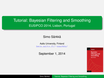
Probabilistic State Space Models: ExampleExample (Gaussian random walk)Gaussian random walk model can be written asxk xk 1 wk 1 , wk 1 N(0, q)yk xk ek ,ek N(0, r ),where xk is the hidden state and yk is the measurement. In terms ofprobability densities the model can be written as 112pexp (xk xk 1 )p(xk xk 1 ) 2q2πq 112 p(yk xk ) exp (yk xk )2r2πrwhich is a discrete-time state space model.Simo SärkkäTutorial: Bayesian Filtering and Smoothing

Probabilistic State Space Models: Example (cont.)Example (Gaussian random walk (cont.))6SignalMeasurement42xk0 2 4 6 8 10020406080100kSimo SärkkäTutorial: Bayesian Filtering and Smoothing

Linear Gaussian State Space ModelsGeneral form of linear Gaussian state space models:qk 1 N(0, Q)xk A xk 1 qk 1 ,rk N(0, R)yk H xk rk ,In probabilistic notation the model is:p(yk xk ) N(yk H xk , R)p(xk xk 1 ) N(xk A xk 1 , Q).Surprisingly general class of models – linearity is frommeasurements to estimates, not from time to outputs.Simo SärkkäTutorial: Bayesian Filtering and Smoothing

Non-Linear State Space ModelsGeneral form of non-linear Gaussian state space models:xk f(xk 1 , qk 1 )yk h(xk , rk ).qk and rk are typically assumed Gaussian.Functions f(·) and h(·) are non-linear functions modeling thedynamics and measurements of the system.Equivalent to the generic probabilistic models of the formxk p(xk xk 1 )yk p(yk xk ).Simo SärkkäTutorial: Bayesian Filtering and Smoothing

Bayesian Optimal Filter: PrincipleBayesian optimal filter computes the distributionp(xk y1:k )Given the following:12Prior distribution p(x0 ).State space model:xk p(xk xk 1 )yk p(yk xk ),3Measurement sequence y1:k y1 , . . . , yk .Computation is based on recursion rule for incorporation of thenew measurement yk into the posterior:p(xk 1 y1:k 1 ) p(xk y1:k )Simo SärkkäTutorial: Bayesian Filtering and Smoothing

Bayesian Optimal Filter: Formal EquationsOptimal filterInitialization: The recursion starts from the prior distribution p(x0 ).Prediction: by the Chapman-Kolmogorov equationZp(xk y1:k 1 ) p(xk xk 1 ) p(xk 1 y1:k 1 ) dxk 1 .Update: by the Bayes’ rulep(xk y1:k ) 1p(yk xk ) p(xk y1:k 1 ).ZkThe normalization constant Zk p(yk y1:k 1 ) is given asZZk p(yk xk ) p(xk y1:k 1 ) dxk .Simo SärkkäTutorial: Bayesian Filtering and Smoothing

Bayesian Optimal Filter: Graphical ExplanationOn prediction step thedistribution of previousstep is propagatedthrough the dynamics.Prior distribution fromprediction and thelikelihood ofmeasurement.Simo SärkkäThe posterior distributionafter combining the priorand likelihood by Bayes’rule.Tutorial: Bayesian Filtering and Smoothing

Kalman Filter: ModelGaussian driven linear model, i.e., Gauss-Markov model:xk Ak 1 xk 1 qk 1yk Hk xk rk ,qk 1 N(0, Qk 1 ) white process noise.rk N(0, Rk ) white measurement noise.Ak 1 is the transition matrix of the dynamic model.Hk is the measurement model matrix.In probabilistic terms the model isp(xk xk 1 ) N(xk Ak 1 xk 1 , Qk 1 )p(yk xk ) N(yk Hk xk , Rk ).Kalman filter computesp(xk y1:k ) N(xk mk , Pk )Simo SärkkäTutorial: Bayesian Filtering and Smoothing

Kalman Filter: EquationsKalman FilterInitialization: x0 N(m0 , P0 )Prediction step:m k Ak 1 mk 1TP k Ak 1 Pk 1 Ak 1 Qk 1 .Update step:vk yk Hk m kTSk Hk P k Hk RkT 1Kk P k Hk Skmk m k Kk vkTPk P k Kk Sk Kk .Simo SärkkäTutorial: Bayesian Filtering and Smoothing

Non-Linear Gaussian State Space ModelBasic Non-Linear Gaussian State Space Model is of the form:xk f(xk 1 ) qk 1yk h(xk ) rkxk Rn is the stateyk Rm is the measurementqk 1 N(0, Qk 1 ) is the Gaussian process noiserk N(0, Rk ) is the Gaussian measurement noisef(·) is the dynamic model functionh(·) is the measurement model functionSimo SärkkäTutorial: Bayesian Filtering and Smoothing

The Idea of Extended Kalman FilterIn EKF, the non-linear functions are linearized as follows:f(x) f(m) Fx (m) (x m)h(x) h(m) Hx (m) (x m)where x N(m, P), and Fx , Hx are the Jacobian matrices of f, h,respectively.Only the first terms in linearization contribute to the approximatemeans of the functions f and h.The second term has zero mean and defines the approximatecovariances of the functions.Can be generalized into approximation of a non-linear transform.Simo SärkkäTutorial: Bayesian Filtering and Smoothing

Linear Approximation of Non-Linear TransformsLinear Approximation of Non-Linear TransformThe linear Gaussian approximation to the joint distribution of x andy g(x) q, where x N(m, P) and q N(0, Q) is P CLxm N,,yµLCTL SLwhereµL g(m)SL Gx (m) P GTx (m) QCL P GTx (m).Simo SärkkäTutorial: Bayesian Filtering and Smoothing

EKF EquationsExtended Kalman filterPrediction:m k f(mk 1 )TP k Fx (mk 1 ) Pk 1 Fx (mk 1 ) Qk 1 .Update:vk yk h(m k) T Sk Hx (m k ) Pk Hx (mk ) Rk 1TKk P k Hx (mk ) Skmk m k Kk vkTPk P k Kk Sk Kk .Simo SärkkäTutorial: Bayesian Filtering and Smoothing

Principle of Unscented Transform [1/4]Problem: Determine the mean and covariance of y:x N(µ, σ 2 )y sin(x)Recall the linearization based approximation:y sin(µ) sin(µ)(x µ) . . . µwhich givesE[y] E[sin(µ) cos(µ)(x µ)] sin(µ)Cov[y] E[(sin(µ) cos(µ)(x µ) sin(µ))2 ] cos2 (µ) σ 2 .Simo SärkkäTutorial: Bayesian Filtering and Smoothing

Principle of Unscented Transform [2/4]Form 3 sigma points as follows:X (0) µX (1) µ σX (2) µ σ.Let’s select some weights W (0) , W (1) , W (2) such that the originalmean and variance can be recovered byXW (i) X (i)µ i2σ XW (i) (X (i) µ)2 .iSimo SärkkäTutorial: Bayesian Filtering and Smoothing

Principle of Unscented Transform [3/4]We use the same formula for approximating the moments ofy sin(x) as follows:Xµ W (i) sin(X (i) )i2σ XW (i) (sin(X (i) ) µ)2 .iFor vectors x N(m, P) the generalization of standard deviation σis the Cholesky factor L P:P L LT .The sigma points can be formed using columns of L (here c is asuitable positive constant):X (0) mX (i) m c LiX (n i) m c LiSimo SärkkäTutorial: Bayesian Filtering and Smoothing

Principle of Unscented Transform [4/4]For transformation y g(x) the approximation is:Xµy W (i) g(X (i) )iΣy XW (i) (g(X (i) ) µy ) (g(X (i) ) µy )T .iIt is convenient to define transformed sigma points:Y (i) g(X (i) )Joint moments of x and y g(x) q are then approximated as X (i) mx(i) X EW µyg(x) qY (i)i xCovg(x) q X (i) (X (i) m) (X (i) m)T(X (i) m) (Y (i) µy )T W(Y (i) µy ) (X (i) m)T (Y (i) µy ) (Y (i) µy )T Q iSimo SärkkäTutorial: Bayesian Filtering and Smoothing

Unscented Transform [1/3]Unscented transformThe unscented transform approximation to the joint distribution of xand y g(x) q where x N(m, P) and q N(0, Q) is P CUxm N,,yµUCTU SUwhere the sub-matrices are formed as follows:1Form the sigma points asX (0) mh iPih i P , m n λX (i) m X (i n) n λiSimo Särkkäi 1, . . . , nTutorial: Bayesian Filtering and Smoothing

Unscented Transform [2/3]Unscented transform (cont.)2Propagate the sigma points through g(·):Y (i) g(X (i) ),3i 0, . . . , 2n.The sub-matrices are then given as:µU SU 2nXi 02nX(m)WiY (i)(c)(Y (i) µU ) (Y (i) µU )T Q(c)(X (i) m) (Y (i) µU )T .Wii 0CU 2nXWii 0Simo SärkkäTutorial: Bayesian Filtering and Smoothing

Unscented Transform [3/3]Unscented transform (cont.)λ is a scaling parameter defined as λ α2 (n κ) n.α and κ determine the spread of the sigma points.(m)Weights Wi(c)and Wi(m)are given as follows:W0 λ/(n λ)(c)W0(m)Wi(c)Wi λ/(n λ) (1 α2 β) 1/{2(n λ)},i 1, . . . , 2n 1/{2(n λ)},i 1, . . . , 2n,β can be used for incorporating prior information on the(non-Gaussian) distribution of x.Simo SärkkäTutorial: Bayesian Filtering and Smoothing

Unscented Kalman Filter (UKF): Algorithm [1/4]Unscented Kalman filter: Prediction step1Form the sigma points:(0)Xk 1 mk 1 ,(i)(i n)Xk 12 hpiPk 1hpii mk 1 n λPk 1 ,Xk 1 mk 1 n λii 1, . . . , n.Propagate the sigma points through the dynamic model:(i)(i)X̂k f(Xk 1 ). i 0, . . . , 2n.Simo SärkkäTutorial: Bayesian Filtering and Smoothing

Unscented Kalman Filter (UKF): Algorithm [2/4]Unscented Kalman filter: Prediction step (cont.)3Compute the predicted mean and covariance:m k P k 2nXi 02nX(m)Wi(c)Wi(i)X̂k(i)(i) T(X̂k m k ) (X̂k mk ) Qk 1 .i 0Simo SärkkäTutorial: Bayesian Filtering and Smoothing

Unscented Kalman Filter (UKF): Algorithm [3/4]Unscented Kalman filter: Update step1Form the sigma points: (0) m k, (i) m k XkXk (i n)Xk2 q P k q i P , m kk n λn λi 1, . . . , n.iPropagate sigma points through the measurement model:(i) (i)Ŷk h(XkSimo Särkkä),i 0, . . . , 2n.Tutorial: Bayesian Filtering and Smoothing

Unscented Kalman Filter (UKF): Algorithm [4/4]Unscented Kalman filter: Update step (cont.)3Compute the following:µk Sk Ck 2nXi 02nXi 02nX(m)Wi(i)Ŷk(c)(Ŷk µk ) (Ŷk µk )T Rk(c)(XkWiWi(i)(i) (i)(i)T m k ) (Ŷk µk )i 0Kk Ck S 1kmk m k Kk [yk µk ]TPk P k Kk Sk Kk .Simo SärkkäTutorial: Bayesian Filtering and Smoothing

Gaussian Moment Matching [1/2]Consider the transformation of x into y:x N(m, P)y g(x).Form Gaussian approximation to (x, y) by directly approximatingthe integrals:ZµM g(x) N(x m, P) dxZSM (g(x) µM ) (g(x) µM )T N(x m, P) dxZCM (x m) (g(x) µM )T N(x m, P) dx.Simo SärkkäTutorial: Bayesian Filtering and Smoothing

Gaussian Moment Matching [2/2]Gaussian moment matchingThe moment matching based Gaussian approximation to the jointdistribution of x and the transformed random variable y g(x) qwhere x N(m, P) and q N(0, Q) is given as P CMxm N,,yµMCTM SMwhereZg(x) N(x m, P) dxµM Z(g(x) µM ) (g(x) µM )T N(x m, P) dx QZ(x m) (g(x) µM )T N(x m, P) dx.SM CM Simo SärkkäTutorial: Bayesian Filtering and Smoothing

Gaussian Filter [1/3]Gaussian filter predictionCompute the following Gaussian integrals:Z mk f(xk 1 ) N(xk 1 mk 1 , Pk 1 ) dxk 1Z TPk (f(xk 1 ) m k ) (f(xk 1 ) mk ) N(xk 1 mk 1 , Pk 1 ) dxk 1 Qk 1 .Simo SärkkäTutorial: Bayesian Filtering and Smoothing

Gaussian Filter [2/3]Gaussian filter update1Compute the following Gaussian integrals:Z µk h(xk ) N(xk m k , Pk ) dxkZ Sk (h(xk ) µk ) (h(xk ) µk )T N(xk m k , Pk ) dxk RkZ TCk (xk m k ) (h(xk ) µk ) N(xk mk , Pk ) dxk .2Then compute the following:Kk Ck S 1kmk m k Kk (yk µk )TPk P k Kk Sk Kk .Simo SärkkäTutorial: Bayesian Filtering and Smoothing

Gaussian Filter [3/3]Special case of assumed density filtering (ADF).Multidimensional Gauss-Hermite quadrature Gauss HermiteKalman filter (GHKF).Cubature integration Cubature Kalman filter (CKF).Monte Carlo integration Monte Carlo Kalman filter (MCKF).Gaussian process / Bayes-Hermite Kalman filter: Form Gaussianprocess regression model from set of sample points and integratethe approximation.Linearization (EKF), unscented transform (UKF), centraldifferences, divided differences can be considered as specialcases.Note that all of these lead to Gaussian approximationsp(xk y1:k ) N(xk mk , Pk )Simo SärkkäTutorial: Bayesian Filtering and Smoothing

Spherical Cubature RulesThe spherical cubature rule is exact up to third degree:Zg(x) N(x m, P) dxZ g(m P ξ) N(ξ 0, I) dξ2n 1 X g(m P ξ (i) ),2ni 1whereξ(i) n ei, i 1, . . . , n n ei n , i n 1, . . . , 2n,where ei denotes a unit vector to the direction of coordinate axis i.A special case of unscented transform!Simo SärkkäTutorial: Bayesian Filtering and Smoothing

Multidimensional Gauss–Hermite RulesCartesian product of classical Gauss–Hermite quadratures givesZg(x) N(x m, P) dxZ g(m P ξ) N(ξ 0, I) dξZZ · · · g(m P ξ) N(ξ1 0, 1) dξ1 · · · N(ξn 0, 1) dξnX W (i1 ) · · · W (in ) g(m P ξ (i1 ,.,in ) ).i1 ,.,inξ (i1 ,.,in ) are formed from the roots of Hermite polynomials.W (ij ) are the weights of one-dimensional Gauss–Hermite rules.Simo SärkkäTutorial: Bayesian Filtering and Smoothing

Particle Filtering: Principle422100 2 1 4 505 2024Animation: Kalman vs. Particle Filtering:Kalman filter animationParticle filter animationSimo SärkkäTutorial: Bayesian Filtering and Smoothing

Sequential Importance Resampling: IdeaSequential Importance Resampling (SIR) ( particle filtering) isconcerned with modelsxk p(xk xk 1 )yk p(yk xk )The SIS algorithm uses a weighted set of particles(i) (i){(wk , xk ) : i 1, . . . , N} such thatE[g(xk ) y1:k ] NX(i)(i)wk g(xk ).i 1Or equivalentlyp(xk y1:k ) NX(i)(i)wk δ(xk xk ),i 1where δ(·) is the Dirac delta function.Uses importance sampling sequentially.Simo SärkkäTutorial: Bayesian Filtering and Smoothing

Sequential Importance Resampling: AlgorithmSequential Importance Resampling(i)Draw point xk from the importance distribution:(i)(i)xk π(xk x0:k 1 , y1:k ),i 1, . . . , N.Calculate new weights(i)(i)(i)wk wk 1(i)(i)p(yk xk ) p(xk xk 1 )(i)(i),i 1, . . . , N,π(xk x0:k 1 , y1:k )and normalize them to sum to unity.If the effective number of particles is too low, perform resampling.Simo SärkkäTutorial: Bayesian Filtering and Smoothing

Sequential Importance Resampling: Bootstrap filterIn bootstrap filter we use the dynamic model as the importancedistribution(i)(i)(i)(i)π(xk x0:k 1 , y1:k ) p(xk xk 1 )and resample at every step:Bootstrap Filter(i)Draw point xk from the dynamic model:(i)(i)xk p(xk xk 1 ),i 1, . . . , N.Calculate new weights(i)(i)wk p(yk xk ),i 1, . . . , N,and normalize them to sum to unity.Perform resampling.Simo SärkkäTutorial: Bayesian Filtering and Smoothing

Sequential Importance Resampling: OptimalImportance DistributionThe optimal importance distribution is(i)(i)(i)(i)π(xk x0:k 1 , y1:k ) p(xk xk 1 , yk )Then the weight update reduces to(i)(i)(i)wk wk 1 p(yk xk 1 ),i 1, . . . , N.The optimal importance distribution can be used, for example,when the state space is finite.Simo SärkkäTutorial: Bayesian Filtering and Smoothing

Sequential Importance Resampling: ImportanceDistribution via Kalman FilteringWe can also form a Gaussian approximation to the optimalimportance distribution:(i)(i)(i)(i)(i)p(xk xk 1 , yk ) N(xk m̃k , P̃k ).by using a single prediction and update steps of a Gaussian filter(i)starting from a singular distribution at xk 1 .We can also replace above with the result of a Gaussian filter(i)(i)N(mk 1 , Pk 1 ) started from a random initial mean.A very common way seems to be to use the previous sample as(i)(i)the mean: N(xk 1 , Pk 1 ).A particle filter with UKF proposal has been given nameunscen

Simo S arkk a Tutorial: Bayesian Filtering and Smoothing. Bayesian Modeling of Dynamics The laws of physics, biology, epidemiology etc.are typically differential equations. Uncertaintiesandunknown sub-phenomenaare modeled as stochastic processes: Physical phenomena: differential equations uncertainty )