WIXLIB

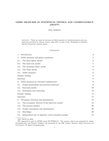
GIBBS MEASURES IN STATISTICAL PHYSICS AND COMBINATORICS(DRAFT)7Figure 4. The monomer-dimer modelWe consider the empty set of edges to be a matching. The size of a matching M , M ,is its number of edges. A perfect matching is a matching that saturates all vertices, that is M V (G) /2.Let M(G) be the set of all matchings of G (we consider the empty set of edges to be amatching). The monomer-dimer model is a random matching M drawn from M(G) accordingto the probability distributionPr[M M ] λ M ,match (λ)ZGwhere M is the number of edges in the matching M and the partition function isXmatchZG(λ) λ M .M M(G)There are many similarities between the hard-core model and the monomer-dimer model;in fact, the monomer-dimer model on G is the hard-core model on the line graph L(G), thegraph with vertex set E(G) and edges between edges of G that share a common vertex.In some important ways, however, the monomer-dimer model is very different than thehard-core model. It is a deep theorem of Heilman and Lieb [31] that the monomer-dimermodel does not exhibit a phase transition on any lattice. The proof uses the Lee-Yang theoryof zeros of partition functions and phase transitions and the result follows from the fact thatall of the roots of the equationmatchZG(λ) 0are real numbers for any graph G. Or in other words, the hard-core partition function ZG (λ)has only real roots as log as G is the line graph of some other graph H. This result wasgeneralized by Chudnovsky and Seymour [10] who showed that ZG (λ) has only real roots forany claw-free graph G; that is, any graph G that avoids an induced star with three leafs.Open Problem. Consider infinite, vertex-transitive graphs. We know that bipartitegraphs with sufficient expansion (eg. Zd ) exhibit a hard-core phase transition. We knowthat line graphs (and claw-free graphs) do not (Heilman-Lieb theorem, Chudnovsky Seymour). What about all the graphs in between? That is, graphs that have claws but whosenumber of ground states is infinite.

8WILL PERKINSFigure 5. The lattice for the discrete hard square model2.4. The Potts model. The Potts model was first studied by Renfrey Potts [43] in his PhDthesis, directed by his advisor Cyril Domb. It is a q-spin generalization of the 2-spin Isingmodel [32] and is an idealization of a magnetic material.For a graph G and an assignment χ of q-colors to each vertex of G, let m(G, χ) denote thenumber of monochromatic edges of G under χ. The Potts model at inverse temperature β isa random q-coloring χ of G chosen according to the distributionPr [χ χ] G,βe βm(G,χ),qZG(β)whereq(β) ZGXe βm(G,χ)χ:V (G) [q]is the q-color Potts model partition function.When β 0 the model is anti-ferromagnetic: colorings with few monochromatic edges arepreferred. When β 0, the model is ferromagnetic: colorings with many monochromaticedges are preferred.2.5. Gibbs measures.Further reading. For an introduction to the hard sphere model by a physicist aimed atmathematicians, see Harmut Löwen’s survey [39]For more on phase transition in systems with hard constraints and their relation to combinatorics, see Brightwell and Winkler [8]For background on the Potts model and its partition function see the surveys of Wu [58]and Sokal [50], and for applications in combinatorics see the survey of Welsh and Morino [57].Exercises.(1) Show that the grand canonical hard sphere partition function on any bounded measurable S satisfies ZS (λ) eλ·vol(S) .

GIBBS MEASURES IN STATISTICAL PHYSICS AND COMBINATORICS(DRAFT)9(2) Compute the hard-core partition function ZSk (λ) for the graph Sk , the star on kleaves. Compute the probability that the center of the star is in the random independent set I.(3) Compute the hard-core partition function ZKd,d (λ) where Kd,d is the complete dregular bipartite graph on 2d vertices.(4) Compute the hard-core partition function ZG (λ) of the cycles C3 , C4 , C5 .(5) Compute the hard-core partition function of the cycle Cn .(6) Prove that the 1-dimensional hard-core model on Z does not exhibit a phase transition, by computing the limiting free energy1f (λ) lim log ZCn (λ)n nand showing that it is a real analytic function of λ.(7) Suppose G is the disjoint union of two graphs H1 and H2 . Show that ZG (λ) ZH1 (λ) · ZH2 (λ).(8) Suppose v is a vertex in some graph with no edges in its neighborhood. Call a vertexu uncovered with respect to an independent set I if N (u) I . Consider thehard-core model on G at fugacity λ and calculate the probability that v is uncoveredgiven that v has exactly j uncovered neighbors.(9) Describe the line graph of the infinite graph Zd .(10) Construct an infinite graph that is claw-free but not the line graph of any graph.(11) Prove that the following is an alternative description of the hard-core model on G. LetI be a random subset of V (G), each vertex included independently with probabilityλ1 λ , conditioned on the event that the vertices form and independent set.3. Gibbs measures in extremal combinatoricsWhile Gibbs measures were originally developed in statistical physics, their mathematicalproperties have proved tremendously useful across many different scientific disciplines, including statistics, computer science, and machine learning where they appear under variousnames including Markov random fields, probabilistic graphical models, Boltzmann distributions, and log-linear models.The majority of this course will focus on how Gibbs measures can be used to prove resultsin extremal graph theory.3.1. Graph polynomials and partition functions. We begin by observing that certainpartition functions from statistical physics arise in graph theory as graph polynomials.The hard-core partition function ZG (λ) is the independence polynomial. The independencepolynomial can also be thought of as the generating function for the sequence i0 (G), i1 (G), . . .where ik (G) denotes the number of independent sets of size k in G:XZG (λ) ik λk .k 0Important parameters in graph theory can be computed using the independence polynomial.For example, ZG (1) counts the total number of independent sets of G, i(G). The order ofthe highest term is the independence number, α(G), the size of the largest independent setof G. The highest order coefficient of the independence polynomial counts the number ofmaximum independent sets in G.

10WILL PERKINSLikewise, the monomer-dimer partition function is the matching generating function (aclose relative of the matching polynomial):XmatchZG(λ) mk (G)λkk 0where mk (G) is the number of matchings of size k in G. The matching number ν(G) is theorder of the highest term. If ν(G) 21 V (G) , then G has a perfect matching, a matchingthat saturates all vertices. In that case m V (G) /2 (G) counts the number of perfect matchingsof G.3.2. Extremal results. The field of extremal combinatorics asks for the maximum and minimum of various graph parameters over different classes of graphs. Some examples of classictheorems from extremal combinatorics are Mantel’s Theorem which answers the questionwhich graph on n vertices containing no triangles has the most edges? (Answer: the complete balanced bipartite graph with n2 /4 edges); or Dirac’s Theorem: which graph on nvertices containing no Hamilton cycle has the largest minimum degree? (Answer: minimumdegree n/2 guarantees a Hamilton cycle; this is tight by taking two disjoint cliques of size n/2each). In Lecture 4 we will discuss an important branch of extremal combinatorics, Ramseytheory.Here we focus on extremal results for bounded-degree graphs.3.2.1. Independent sets in regular graphs. Which d-regular graph has the most independentsets? This question was first raised in the context of number theory by Andrew Granville, andthe first approximate answer was given by Noga Alon [2] who applied the result to problemsin combinatorial group theory.Jeff Kahn gave a tight answer in the case of d-regular bipartite graphs.Theorem 1 (Kahn [35]). Let 2d divide n Then for any d-regular, bipartite graph G on nvertices, n/2di(G) i(Hd,n ) 2d 1 1,where Hd,n is the graph consisting of n/2d copies of Kd,d .In terms of the independence polynomial, we can rephrase this as: for any d-regular,bipartite G,ZG (1) ZKd,d (1)n/2d .Kahn’s proof is via the entropy method. Recall the entropy of a discrete random variableY:H(Y ) XPr[Y y] log Pr[Y y] .ySee Appendix B.2 for the basics of entropy from information theory. See also Galvin’s lecturenotes on the entropy method [27] for an exposition of Theorem 1 and extensions. The maintool we will use is Shearer’s Lemma.

GIBBS MEASURES IN STATISTICAL PHYSICS AND COMBINATORICS(DRAFT)11Lemma 2 (Shearer’s Lemma [11]). Let F be a family of subsets of [n] {1, . . . n} so thateach element i [n] is contained in at least t sets of F. For a (random) vector (X1 , . . . Xn )and a set F [n], let XF (Xi )i F . Then1 XH(X1 , . . . Xn ) H(XF ) .tF FProof of Theorem 1. Let G be a d-regular, n vertex graph with bipartition (L, R). Let I bean independent set chosen uniformly from all the independent sets of G. Since I is uniform,we haveH(I) log i(G) ,and so we aim to showH(I) nlog 2d 1 1 .2dOrder the vertices of G v1 , . . . vn with the first n/2 in L and the rest in R. We can expressthe random independent set I as a random vector of 0’s and 1’s, (X1 , . . . Xn ) where Xi 1 ifvi I. Let XL (X1 , . . . Xn/2 ) and XR (Xn/2 1 , . . . Xn ). For a vertex v, XN (v) denotesXu1 , . . . Xud where u1 , . . . ud are the neighbors of v. By the Chain Rule for entropy we haveH(I) H(X1 , . . . Xn ) H(XL ) H(XL XR ) H(X1 , . . . Xn ) H(XL ) n/2XH(Xi XN (vi ) )i 1by subadditivity and monotonicity of conditioning. Now we can apply Shearer’s Lemma toH(XL ) with the family of sets F being the neighborhoods N (v1 ), . . . N (vn/2 ); each i [n/2]is covered by exactly d sets since G is d-regular. This givesH(I) (1)n/2X1i 1dH(XN (vi ) ) H(Xi XN (vi ) ) .Now we bound each term by conditioning on the event that vi is uncovered, that is, N (v) I . Let q(vi ) Pr[N (vi ) I ]. ThenH(XN (vi ) ) q(vi ) log q(vi ) (1 q(vi )) log(1 q(vi )) (1 q(vi ))H(XN (vi ) N (v) I ) d 12 1 (1 q(vi )) log q(vi ) logq(vi )1 q(vi )using the bound H(Y) log ( support(Y) ) in the last step. We can also writeH(Xi XN (vi ) ) q(vi ) log(2) .Putting these together gives H(XN (vi ) ) d · H(Xi XN (vi ) ) q(vi ) · log2dq(vi ) log(2d 1 1) (1 q(vi )) · log2d 11 q(vi ) by Jensen’s Inequality .Substituting this back into (1), we obtainH(I) as desired.nlog(2d 1 1)2d

12WILL PERKINS3.2.2. Bregman’s Theorem.Theorem 3 (Bregman [7]). Let A be an n n matrix with {0, 1}-valued entries and rowsums d1 , . . . dn . ThennYperm(A) (di !)1/di .i 1Let mperf (G) denote the number of perfect matchings of a graph G.Corollary 4. Suppose G is a bipartite graph on two parts of n/2 vertices each, with leftdegrees d1 , . . . dn/2 , thenn/2Ymperf (G) (di !)1/di .i 1In particular, if 2d divides n, and G is a d-regular bipartite graph, thenmperf (G) mperf (Hd,n ).In the case of d-regular bipartite graphs, Bregman’s theorem states thatmperf (G) mperf (Kd,d )n/2d .Proof of Theorem 3. The proof we present is due to Radhakrishnan [44]. Let G be a bipartitegraph on two sets (L, R) of n/2 vertices each with left degrees d1 , . . . dn/2 . Let M be auniformly random perfect matching from G.Suppose V (G) L R with L {u1 , . . . un/2 } and R {v1 , . . . vn/2 }. We view a perfectmatching in G as a permutation σ of [n/2] so that (ui , vσ(i) ) E(G). Let S be the set of allsuch σ and let σ be a uniformly random element of S.Since σ is chosen uniformly from S, and S mperf (G), we havelog mperf (G) H(σ) .So our goal is to prove the upper boundH(σ) n/2Xlog di !i 1di.Let τ be a permutation of [n/2]. Then we will uncover the permutation σ in the orderdetermined by τ :σ(τ (1)), σ(τ (2)), . . . σ(τ (n/2)) .By the chain rule of entropy, we haveH(σ) n/2XH(σ(τ (i)) σ(τ (1)), . . . σ(τ (i 1))) .i 1Since this is true for every τ , we can take the expectation over a uniformly random τ .H(σ) n/2Xi 1Eτ H(σ(τ (i)) σ(τ (1)), . . . σ(τ (i 1))) .

GIBBS MEASURES IN STATISTICAL PHYSICS AND COMBINATORICS(DRAFT)13For τ and i fixed, let k be such that τ (k) i. Then we can writeH(σ) n/2XEτ H(σ(i) σ(τ (1)), . . . σ(τ (k 1))) .i 1Now let Ri (σ, τ ) be the number of neighbors of ui that have not be revealed byσ(τ (1)), . . . σ(τ (k 1)). Then using the fact that H(Y ) log supp(Y ) ,H(σ) n/2XEτdiXi 1 j 1n/2 diXXi 1 j 1Pr[ Ri (σ, τ ) j] log jσPr [ Ri (σ, τ ) j] log j .σ,τNow for any fixed σ, Prτ [ Ri (σ, τ ) j] 1/di by symmetry, and son/2diX1 Xlog jH(σ) dii 1 j 1n/2Xlog di !i 1dias desired. 3.3. Extensions and reductions. Galvin and Tetali [29] proved a very broad generalizationof Kahn’s result. To describe it we need a definition.Definition. Let G and H be two finite graphs. A map φ : V (G) V (H) is a homomorphism from G to H if for every (u, v) E(G), (φ(u), φ(v)) E(H). Let hom(G, H) denotethe number of homomorphisms from G to H.Example. Suppose H ind is the graph on two vertices w1 , w2 , with an edge between w1 andw2 and a self-loop on w2 . Then homomorphisms from G to H ind correspond to independentsets, with the vertices of the independent set given by φ 1 (w1 ), and so hom(G, H ind ) i(G),the number of independent sets of G.Example. Homomorphisms from G to Kq , the complete graph on q vertices, correspond toproper q-colorings of V (G).Jeff Kahn’s result on independent sets can be restated as the fact thathom(G, H ind ) hom(Kd,d , H ind )n/2dfor any d-regular, bipartite G. What Galvin and Tetali show is that this result holds incomplete generality over the choice of the target graph H, at least over bipartite regulargraphs.Theorem 5. Let H be any graph, with or without self-loops, and let G be any d-regular,bipartite graph. Thenhom(G, H) hom(Kd,d , H)n/2d .

14WILL PERKINSTheorem 6 (Kahn [35], Galvin-Tetali [29], Zhao [59]). For any d-regular graph G and anyλ 0,11log ZG (λ) log ZKd,d (λ). V (G) 2dRemoving the bipartite restriction, as Zhao did for independent sets, is not possible ingeneral. (For a simple example see the exercises). Zhao [60] found a large family of Hfor which the statement for general d-regular graphs reduces to the bipartite statement.Sernau [47] found a large such family and disproved a conjecture of Galvin [26] that eitherKd,d or Kd 1 is always the maximizing graph.One specific target graph H that arises in statistical physics is H WR , the graph on threevertices, w1 , w2 , w3 , each with a self-loop, and w2 joined to both w1 and w3 . Homomorphismsfrom G to H WR correspond to valid configurations in the Widom-Rowlinson model in whichparticles of two different types can occupy sites on a lattice, but particles of different typesare forbidden from neighboring each other. (The vertices w1 and w3 correspond to the twodifferent types, while w2 corresponds to an empty site). The extremal graph for WidomRowlinson configurations is the clique.Theorem 7 (Cohen, Perkins, Tetali [13]; Sernau [47]). For all d-regular G,hom(G, H WR ) hom(Kd 1 , H WR )n/(d 1) .This theorem was first proved with the methods of Section 4, but it was later observed [12,47] that it follows from a reduction from the case of independent sets.Perhaps the most outstanding unresolved case of target graph H is that of proper colorings(H Kq ). Galvin and Tetali conjectured that a union of Kd,d ’s maximize the number ofq-colorings over all d-regular graphs.Conjecture 8 (Galvin, Tetali [29]). For all d-regular G, and all q 2,hom(G, Kq ) hom(Kd,d , Kq )n/2d .Galvin and Tetali prove this for bipartite G with their general theorem. Partial resultstowards this conjecture have been proved [60, 26, 28]. Recently the case d 3 and arbitraryq was resolved [23]. The proof proceeds via the Potts model from statistical physics; we willreturn to this in Lecture 5.Further reading. Zhao wrote a recent survey on extremal problems for homomorphismcounts in regular graph [61]. See also Csikvári [17] for further results and open problems inthis area.Exercises.(1) Let H be the graph consisting of two vertices each with self loops but no edge joiningthe two. Show that hom(Kd 1 , H)1/(d 1) hom(Kd,d , H)1/2d .(2) Let G be any graph. Let G K2 be the bipartite double cover of G. That is, G K2has vertex set V (G) {0, 1} with an edge between (u, i) and (v, j) if uv E(G) andi 0, j 1 or i 1, j 0. Prove thati(G)2 i(G K2 ).Deduce that Kahn’s theorem on independent sets in d-regular bipartite graphs canbe extended to all d-regular graphs. This is Zhao’s proof [59].

GIBBS MEASURES IN STATISTICAL PHYSICS AND COMBINATORICS(DRAFT)15(3) Prove (in an elementary way) that for all d-regular G on n vertices,in/2 (G) id (Kd,d )n/2d .(4) For a given indpendent set I and a specified vertex v V (G), let us say that aneighbor u of v is externally uncovered if no neighbor of u that is a second neighborof v is in I. What is the probability that a vertex v is uncovered, given that thesubgraph induced by its externally uncovered neighbors is isomorphic to a graph H?M (λ) Z M (λ) for all(5) Let G, H be two graphs on n vertices each. Prove that if ZGHλ 0, then mperf (G) mperf (H).(6) By going through the proof of Theorem 1, show that equality in the theorem isattained only by Kd,d or Hd,n .4. Occupancy fractions and optimizationIn this section we present a new approach to proving extremal theorems for sparse graphs.We will prove extremal results for partition functions and graph polynomials by optimizingthe logarithmic derivative of a given partition function over a given class of graphs. Byintegrating we obtain the corresponding result for the partition function. The logarithmicderivative has a probabilistic interpretation as the expectation of an observable of the relevantmodel from statistical physics, and so working directly with the model we impose localprobabilistic constraints bases on the graph structure and parameters of the model, then relaxthe optimization problem to all local probability distributions satisfying these constraints.An observable of a Gibbs measure is simply a random variable, a function of the randomconfiguration. One particularly important observable is the energy. In general we can describe a Gibbs distribution in terms of a Hamiltonian, or energy function, H(σ) mappingconfigurations to real numbers. We then writePr[σ σ] e βH(σ),Z(β)where β is called the inverse temperature and the partition function Z(β) again the normalizing constant.Pσe βH(σ) isThe energy of the random configuration H(σ) is one example of an observable. Theexpectation of this observable isXEβ H(σ) H(σ) Pr[σ σ]βσ XσH(σ)e βH(σ )Z(β)Z 0 (β)Z(β) (log Z(β))0 . This simple calculation is the key to the method that follows.4.1. The occupancy fraction of the hard-core model. We start with independent setsand the hard-core model, where the relevant observable is the occupancy fraction.

16WILL PERKINSDefinition 9. The occupancy fraction of the hard-core model on a graph G at fugacity λ isthe expected fraction of vertices that appear in the random independent set:1αG (λ) EG,λ I . V (G) We begin by collecting some basic facts about the occupancy fraction.Proposition 10. The occupancy fraction is λ times the derivative of the free energy: 01αG (λ) λ ·log ZG (λ) . V (G) Proof. We write1EG,λ I V (G) X1 I · Pr [I

Abstract. These are notes for lectures on Gibbs measures in statistical physics and com-binatorics presented in Athens, Greece, May 2017, as part of the 'Techniques in Random Discrete Structures' summer school. Contents 1. Introduction 2 2. Gibbs measures and phase transitions 2 2.1. The hard sphere model 2 2.2. The hard-core model 5 2.3.