WIXLIB

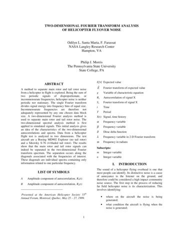
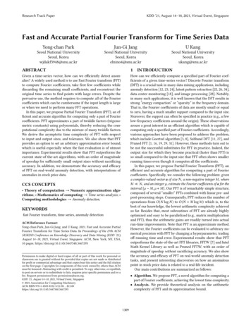
Research Track PaperPFT (proposed) Pruned FFTRunning time (ms)10. Ｘ 1.Ｘ 0.1Ｘ Ｘ Ｘ Ο Ο Ο0.01 ＸΟΟ 212214216Ｘ Ｘ ΟΟ218ΟＸ ΟΟΟ32Ｘ Ｘ 19 220222Running time (ms)ΟKDD ’21, August 14–18, 2021, Virtual Event, SingaporeＸ FFTW ΟＸ Ｘ Ｘ Ｘ Ｘ Ｘ Ｘ Ｘ Ｘ Ｘ Ｘ16 Ο810.2 4ΟΟ21Ο Ο Ο210Input size(a) Running time vs. input sizeTable 1: Table of symbols. MKL212ΟΟ Ο214Ο216218220Output size(b) Running time vs. output sizeFigure 1: (a) Running time vs. input size for target range 𝑅0,2922with {S𝑛 }𝑛 12datasets, and (b) running time vs. output sizefor fixed input size 222 . We set the precision of all the methodsthe same, by making the relative error strictly less than 10 6 .Note that PFT significantly outperforms competitors whenthe output size is smaller than the input size, which is exactlyour target task.𝜔𝑛𝒂ˆˆE ( 𝒂)𝑁𝑀𝜇𝑅 𝜇,𝑀𝑝, 𝑞𝑟𝜖 · 𝑅𝑃𝛼𝑛-th primitive root of unityFourier coefficient of 𝒂estimated Fourier coefficient of 𝒂input size descriptoroutput size descriptorcenter of target rangetarget range [𝜇 𝑀, 𝜇 𝑀] Zdivisors of 𝑁number of approximating termstoleranceuniform norm restricted to 𝑅 Rset of polynomials on R of degree at most 𝛼best polynomial approximation to 𝑒𝑢𝑖𝑥 out of 𝑃𝛼under restriction 𝑥 𝜉 sup{𝜉 0 : P𝑟 1,𝜉,𝜋 (𝑥) 𝑒 𝜋𝑖𝑥 𝑥 𝜉 𝜖}𝑗-th coefficient of P𝑟 1,𝜉 (𝜖,𝑟 ),𝜋𝜉 (𝜖, 𝑟 )𝑤𝜖,𝑟,𝑗RELATED WORKSWe describe the related works on this paper.2.1DefinitionP𝛼,𝜉,𝑢 Speed and Accuracy. PFT shows state-of-the-art speed on bothsynthetic and real-world datasets without sacrificing accuracy(see Figure 1). Application. We conduct anomaly detection on real-world datasets,and present discovery results verifying that our algorithm accurately and quickly finds anomalies.Table 1 summarizes the symbols used. The code and datasets areavailable at https://github.com/snudatalab/PFT.2SymbolExisting MethodsWe describe various existing approaches for computing partialFourier coefficients, and compare them with our proposed method.Fast Fourier transform. One may consider just using FastFourier transform (FFT) and discarding the unnecessary coefficients, where FFT efficiently computes the full DFT, reducing thearithmetic cost from naïve 𝑂 (𝑁 2 ) to 𝑂 (𝑁 log 𝑁 ). Such an approachhas two major advantages: (1) it is straightforward to implement,and (2) the method often outperforms the competitors because it directly employs FFT which has been highly optimized over decades.Therefore, we provide extensive comparisons of PFT and FFT boththeoretically and experimentally. In particular, we show that PFToutperforms the FFT by orders of magnitude when the output sizeis small enough ( 10%) compared to the input size (Section 4.2).Goertzel algorithm. Goertzel algorithm [3, 8] is one of the firstmethods devised for computing only a part of Fourier coefficients.The technique is essentially the same as computing the individualcoefficients of DFT, thus requiring 𝑂 (𝑀𝑁 ) operations for 𝑀 coefficients of an input with size 𝑁 . Specifically, theoretical analysisrepresents “the 𝑀 at which the Goertzel algorithm is advantageousover FFT” as 𝑀 2 log 𝑁 [32]. For example, with 𝑁 222 , theGoertzel algorithm becomes faster than FFT only when 𝑀 44,while PFT outperforms FFT for 𝑀 219 524288 (Figure 1(b)).1310A few variants which improve the Goertzel algorithm have beenproposed [2]. Nevertheless, the performance gain is only by a smallconstant factor, thus they are still limited to rare scenarios where avery few number of coefficients are required.Subband DFT. Subband DFT [11, 27] consists of two stagesof algorithm: Hadamard transform that decomposes the input sequence into a set of smaller subsequences, and correction stage forrecombination. The algorithm approximates a part of coefficientsby eliminating subsequences with small energy contribution, andmanages to reduce the number of operations to 𝑂 (𝑁 𝑀 log 𝑁 ).Apart from the arithmetic gain, however, there is a substantial issueof low accuracy with the Subband DFT. Indeed, experimental results[11] show that the relative approximation error of the method isaround 10 1 (only one significant figure) regardless of output size.Moreover, with PFT, the Fourier coefficients can be evaluated to arbitrary numerical precision, which is not the case for Subband DFT.Such limitations often preclude one from considering the SubbandDFT in applications that require a certain degree of accuracy.Pruned FFT. FFT pruning [1, 16, 19, 29, 31] is another techniquefor the efficient computation of partial Fourier coefficients. Themethod is a modification of the standard split-radix FFT, where theedges (operations) in a flow graph are pruned away if they do notaffect the specified range of frequency domain. Besides being almostoptimized (it uses FFT as a subroutine), the FFT pruning algorithmis exact and reduces the arithmetic cost to 𝑂 (𝑁 log 𝑀). Thus, alongwith the full FFT, the pruned FFT is reasonably the most appropriatecompetitor of our proposed method. Through experiments (Section4.2), we show that PFT consistently outperforms the pruned FFT,significantly extending the range of output sizes for which partialFourier transform becomes practical.Finally, we mention that there have been other approaches butwith different settings. For example, [9, 10] and [13] propose SparseFourier transform, which estimates the top-𝑘 (the 𝑘 largest in magnitude) Fourier coefficients of a given vector. The algorithm is usefulwhen there is prior knowledge of the number of non-zero coefficients in frequency domain. Note that our setting does not requireany prior knowledge of the given data.

Research Track Paper2.2KDD ’21, August 14–18, 2021, Virtual Event, SingaporeApplications of FFTapproximating terms), enabling fine-tuning the output range andthe approximation bound of the estimation. Our first goal is to finda collection of twiddle factors with small oscillations. This can beachieved by slightly adjusting the summand of DFT and splittingthe summation as in the Cooley-Tukey algorithm (Section 3.1.1).Next, using a proper base exponential function, we give an explicitform of approximation to the twiddle factors (Section 3.1.2).We outline various applications of Fast Fourier transform, to whichpartial Fourier transform can potentially be applied. FFT has beenwidely used for anomaly detection [12, 23, 24]. [12] and [24] detectanomalous points of a given data by extracting a compact representation using Spectral Residual (SR) based on FFT. [23] uses FFT todetect local spatial outliers which have similar patterns within aregion but different patterns from the outside. FFT also serves asthe basis for discovering latent patterns [22, 26, 34]. [34] employsFFT to model multi-frequency trading patterns from past marketdata for stock price prediction. [26] presents an FFT-based approachfor automatic sleep stage scoring and apnea-hypopnea detectionby extracting meaningful features from EGG, ECG, EOG and EMGdata. [22] attempts to detect fake news by designing a CNN-basednetwork that captures the complex patterns of fake images in thefrequency domain. Several works [15, 20, 21, 33] exploit FFT forefficient operations. [20] leverages FFT to efficiently compute apolynomial kernel used with support vector machines (SVMs). [15]proposes an efficient Tucker decomposition method using FFT, and[33] applies FFT to a circulant linear system for seasonal-trenddecomposition. In addition, FFT has been used for fast training ofconvolutional neural networks [17, 25] and an efficient recommendation model on a heterogeneous graph [14].33.1.1 Smooth Twiddle Factors. Recall that the DFT of a complexvalued vector 𝒂 of size 𝑁 is defined as follows: ︁𝑎ˆ𝑚 𝑎𝑛 𝜔𝑚𝑛(1)𝑁 ,𝑛 [𝑁 ]where 𝜔 𝑁 𝑒 2𝜋𝑖/𝑁 is the 𝑁 -th primitive root of unity, and [𝑁 ]denotes {0, 1, · · · , 𝑁 1} (in this paper, we follow the conventionof viewing a vector 𝒗 (𝑣 0, 𝑣 1, · · · , 𝑣 𝑁 1 ) of size 𝑁 as a finitesequence defined on [𝑁 ]). Assume that 𝑁 𝑝𝑞 for two integers𝑝, 𝑞 1. The Cooley-Tukey algorithm [5] re-expresses (1) as ︁ ︁ ︁ ︁𝑚 (𝑞𝑘 𝑙)𝑚𝑘𝑎ˆ𝑚 𝑎𝑞𝑘 𝑙 𝜔 𝑁 𝑎𝑞𝑘 𝑙 𝜔𝑚𝑙𝑁 𝜔 𝑝 , (2)𝑘 [𝑝 ] 𝑙 [𝑞 ]yielding two collections of twiddle factors, namely {𝜔𝑚𝑙𝑁 }𝑙 [𝑞 ] and𝑚𝑘{𝜔 𝑝 }𝑘 [𝑝 ] . Consider the problem of computing 𝑎ˆ𝑚 for 𝑀 𝑚 𝑀, where 𝑀 𝑁 /2 is a non-negative integer. In this case, note that 2𝜋𝑖𝑚𝑙/𝑁 ranges from 2𝜋𝑖𝑀 (𝑞 1)/𝑁the exponent of 𝜔𝑚𝑙𝑁 𝑒 2𝜋𝑖𝑚𝑘/𝑝 rangesto 2𝜋𝑖𝑀 (𝑞 1)/𝑁 and the exponent of 𝜔𝑚𝑘𝑝 𝑒PROPOSED METHODWe propose PFT, an efficient and accurate algorithm for computinga specified part of Fourier coefficients. The main challenges andour approaches are as follows:(𝑞 1)/𝑁from 2𝜋𝑖𝑀 (𝑝 1)/𝑝 to 2𝜋𝑖𝑀 (𝑝 1)/𝑝. Here (𝑝 1)/𝑝 𝑝1 , meaning that the first collection contains smoother twiddle factors compared to the second one. Typically, a smoother function results in abetter approximation via polynomials. In this sense, it is reasonableto approximate the first collection of twiddle factors in (2) withpolynomial functions, thereby reducing the complexity of the computation due to the mixture of two collections of twiddle factors.Indeed, one can further reduce the complexity of approximation:we slightly adjust the summand in (2) as follows. ︁ ︁𝑚 (𝑙 𝑞/2) 𝑚𝑘𝑎ˆ𝑚 𝜔𝑚𝑎𝑞𝑘 𝑙 𝜔 𝑁𝜔𝑝 .(3)2𝑝(1) How can we extract essential information for a specifiedoutput? Considering that only a specified part of coefficientsare needed, we should find an algorithm requiring fewer operations than the direct use of conventional FFT. This is achievableby carefully modifying the Cooley-Tukey algorithm, findingsmooth twiddle factors (trigonometric factors), and approximating them using polynomials (Section 3.1.1).(2) How can we reduce approximation cost? The approachgiven above involves an approximation process, which wouldbe computationally demanding. We propose using a base exponential function, by which all data-independent factors canbe precomputed, enabling one to bypass the approximationproblem during the run-time (Sections 3.1.2 and 3.2).(3) How can we further reduce numerical computation? Wecarefully reorder the operations and factorize the terms in orderto alleviate the complexity of PFT. Such techniques separate alldata-independent factors from data-dependent factors, allowingfurther precomputation. The arithmetic cost of the resultingalgorithm is 𝑂 ((𝑁 𝑀 log 𝑀) log(1/𝜖)), where 𝑁 and 𝑀 are input and output size descriptors, respectively, and 𝜖 is a tolerance(Sections 3.3 and 3.4).3.1𝑘 [𝑝 ] 𝑙 [𝑞 ]𝑘 [𝑝 ] 𝑙 [𝑞 ]In (3), we observe that the range of exponents of the first collec𝑚 (𝑙 𝑞/2)tion {𝜔 𝑁}𝑙 [𝑞 ] of twiddle factors is [ 𝜋𝑖𝑀/𝑝, 𝜋𝑖𝑀/𝑝], acontraction by a factor of around 2 when compared with the previous [ 2𝜋𝑖𝑀 (𝑞 1)/𝑁 , 2𝜋𝑖𝑀 (𝑞 1)/𝑁 ], hence even smoothertwiddle factors. There is an extra twiddle factor 𝜔𝑚2𝑝 in (3). Notethat, however, it depends on neither 𝑘 nor 𝑙, so the amount of theadditional computation is relatively small.3.1.2 Base Exponential Function. The first collection of twiddlefactors in (3) consists of 𝑞 distinct exponential functions. One canapply approximation process for each function in the collection;however, this would be time-consuming. A more plausible approachis to 1) choose a base exponential function 𝑒𝑢𝑖𝑥 for a fixed 𝑢 R,2) approximate 𝑒𝑢𝑖𝑥 using a polynomial, and 3) exploit a propertyof exponential functions: the laws of exponents. Specifically, suppose that we obtained a polynomial P (𝑥) that approximates 𝑒𝑢𝑖𝑥on 𝑥 𝜉 , where 𝑢, 𝜉 R \ {0}. Consider another exponentialfunction 𝑒 𝑣𝑖𝑥 , where 𝑣 0. Since 𝑒 𝑣𝑖𝑥 𝑒𝑢𝑖 (𝑣𝑥/𝑢) , the re-scaledApproximation of Twiddle FactorsThe key of our algorithm is to approximate a part of smooth (lessoscillatory) twiddle factors by using polynomial functions, reducingthe computational complexity of DFT due to the mixture of manytwiddle factors. Using polynomial approximation also allows oneto carefully control the degree of polynomial (or the number of1311

Research Track PaperKDD ’21, August 14–18, 2021, Virtual Event, Singaporepolynomial P (𝑣𝑥/𝑢) approximates 𝑒 𝑣𝑖𝑥 on 𝑥 𝑢𝜉/𝑣 . This observation indicates that once we find an approximation P to 𝑒𝑢𝑖𝑥on 𝑥 𝜉 for properly selected 𝑢 and 𝜉, all elements belong𝑚 (𝑙 𝑞/2)ing to {𝜔 𝑁 𝑒 2𝜋𝑖𝑚 (𝑙 𝑞/2)/𝑁 }𝑙 [𝑞 ] can be approximatedby re-scaling P. Fixing a base exponential function also enablesprecomputing a polynomial that approximates it, so that one canbypass the approximation problem during the run-time. We further elaborate this idea in a rigorous manner after giving a fewdefinitions (see Definitions 3.1 and 3.2).Let · 𝑅 be the uniform norm (or supremum norm) restrictedto a set 𝑅 R, that is, 𝑓 𝑅 sup{ 𝑓 (𝑥) : 𝑥 𝑅} and 𝑃𝛼 be theset of polynomials on R of degree at most 𝛼.given method works only when our target range is centered at𝜇 0. A slight modification of the algorithm allows the targetrange to be arbitrarily centered. One possible approach is as follows: given a complex-valued vector 𝒙 of size 𝑁 , we define 𝒚 as𝜇𝑛𝑦𝑛 𝑥𝑛 · 𝜔 𝑁 . Then, the Fourier coefficients of 𝒙 and 𝒚 satisfy thefollowing relationship (called Shift Theorem): ︁ ︁𝜇𝑛(𝑚 𝜇)𝑛𝑦ˆ𝑚 𝑥𝑛 𝜔 𝑁 𝜔𝑚𝑛𝑥𝑛 𝜔 𝑁 𝑥ˆ𝑚 𝜇 .𝑁 𝑛 [𝑁 ]Definition 3.1. Given a non-negative integer 𝛼 and non-zero realnumbers 𝜉, 𝑢, we define a polynomial P𝛼,𝜉,𝑢 as the best approximation to 𝑒𝑢𝑖𝑥 out of the space 𝑃𝛼 under the restriction 𝑥 𝜉 :Lemma 1. Given a non-negative integer 𝛼, non-zero real numbers𝜉, 𝑢, and a real number 𝜇, the following equality holds:P𝛼,𝜉,𝑢 : arg min 𝑃 (𝑥) 𝑒𝑢𝑖𝑥 𝑥 𝜉 ,𝑃 𝑃𝛼and P𝛼,𝜉,𝑢 1 when 𝜉 0 or 𝑢 0.𝑒𝑢𝑖𝜇 · P𝛼,𝜉,𝑢 (𝑥 𝜇) arg min 𝑃 (𝑥) 𝑒𝑢𝑖𝑥 𝑥 𝜇 𝜉 . 𝑃 𝑃𝛼[30] proved the unique existence of P𝛼,𝜉,𝑢 , and a few techniquescalled minimax approximation algorithms for computing the polynomial are reviewed in [6]. Proof. See Supplement A.1.This observation implies that, in order to obtain a polynomialapproximating 𝑒𝑢𝑖𝑥 on 𝑥 𝜇 𝜉 , we first find a polynomialP approximating 𝑒𝑢𝑖𝑥 on 𝑥 𝜉 , then translate P by 𝜇 andmultiply it with the scalar 𝑒𝑢𝑖𝜇 . Applying this process to the previously obtained approximation polynomials (see Section 3.1.2) yields𝜇 (𝑙 𝑞/2){𝜔 𝑁· P𝑟 1,𝜉 (𝜖,𝑟 ),𝜋 ( 2(𝑚 𝜇)(𝑙 𝑞/2)/𝑁 )}𝑙 [𝑞 ] . We substi-Definition 3.2. Given a tolerance 𝜖 0 and a positive integer𝑟 1, we define 𝜉 (𝜖, 𝑟 ) to be the scope about the origin such thatthe exponential function 𝑒 𝜋𝑖𝑥 can be approximated by a polynomialof degree less than 𝑟 with approximation bound 𝜖:𝑚 (𝑙 𝑞/2)𝜉 (𝜖, 𝑟 ) : sup{𝜉 0 : P𝑟 1,𝜉,𝜋 (𝑥) 𝑒 𝜋𝑖𝑥 𝑥 𝜉 𝜖}.tute them for {𝜔 𝑁}𝑙 [𝑞 ] in (3), which gives the followingestimation of 𝑎ˆ𝑚 for 𝑚 𝑅 𝜇,𝑀 , where 𝑘 [𝑝], 𝑙 [𝑞], and 𝑗 [𝑟 ]: ︁𝜇 (𝑙 𝑞/2)𝜔𝑚𝑎𝑞𝑘 𝑙 𝜔 𝑁P𝑟 1,𝜉 (𝜖,𝑟 ),𝜋 ( 2(𝑚 𝜇)(𝑙 𝑞/2)/𝑁 ) 𝜔𝑚𝑘𝑝2𝑝We express the corresponding polynomial as P𝑟 1,𝜉 (𝜖,𝑟 ),𝜋 (𝑥) Í𝑗 𝑗 [𝑟 ] 𝑤 𝜖,𝑟,𝑗 · 𝑥 .In Definition 3.2, we choose 𝑒 𝜋𝑖𝑥 as a base exponential function. The rationale behind is as follows. First, using a minimaxapproximation algorithm, we precompute 𝜉 (𝜖, 𝑟 ) and {𝑤𝜖,𝑟,𝑗 } 𝑗 [𝑟 ]for several tolerance 𝜖’s (e.g. 10 1, 10 2, · · · ) and positive integer𝑟 ’s (typically 𝑟 25). When 𝑁 , 𝑀, 𝑝 and 𝜖 are given, we findthe minimum 𝑟 satisfying 𝜉 (𝜖, 𝑟 ) 𝑀/𝑝. Then, by the preceding argument, it follows that the re-scaled polynomial functionP𝑟 1,𝜉 (𝜖,𝑟 ),𝜋 ( 2𝑥 (𝑙 𝑞/2)/𝑁 ) approximates 𝑒 2𝜋𝑖𝑥 (𝑙 𝑞/2)/𝑁 on𝑁 𝑥 2(𝑙 𝑞/2)·𝑀𝑝 for each 𝑙 [𝑞] (note that if 𝑙 𝑞/2 0, we𝑘,𝑙𝜇 (𝑙 𝑞/2) 𝜔𝑚2𝑝 ︁ 𝜔𝑚2𝑝 ︁ ︁𝑎𝑞𝑘 𝑙 𝜔 𝑁𝑗 ︁𝑤𝜖,𝑟,𝑗 ( 2(𝑚 𝜇)(𝑙 𝑞/2)/𝑁 ) 𝑗 𝜔𝑚𝑘𝑝𝑗𝑘,𝑙𝜇 (𝑙 𝑞/2)𝑎𝑞𝑘 𝑙 𝜔 𝑁𝑤𝜖,𝑟,𝑗 ((𝑚 𝜇)/𝑝) 𝑗 (1 2𝑙/𝑞) 𝑗 𝜔𝑚𝑘𝑝 .𝑘,𝑙(5)3.3Efficient SummationsWe have found that three main summation steps (each being over𝑗, 𝑘, and 𝑙) take place when computing the partial Fourier coeffiÍcients. Note that in (5), the innermost summation 𝑗 is movedto the outermost position, and the term 2(𝑚 𝜇)(𝑙 𝑞/2)/𝑁 isfactorized into two independent terms, (𝑚 𝜇)/𝑝 and 1 2𝑙/𝑞.Interchanging the order of summations and factorizing the termresult in a significant computational benefit; we elucidate whatoperator we should utilize for each summation and how we cansave the arithmetic costs from it. As we will see, the innermost sumover 𝑙 corresponds to a matrix multiplication, the second sum over𝑘 can be viewed as a set of DFTs, and the outermost sum over 𝑗is an inner product. For the first sum, let 𝐴 (𝑎𝑘,𝑙 ) 𝑎𝑞𝑘 𝑙 and𝑞𝑁𝑁𝑀have 2(𝑙 𝑞/2)·𝑀𝑝 ). Here 2(𝑙 𝑞/2) · 𝑝 2𝑙 𝑞 · 𝑀 𝑀for all 𝑙 [𝑞]. Therefore, we obtain a polynomial approximation𝑚 (𝑙 𝑞/2)on 𝑚 𝑀 for each twiddle factor in {𝜔 𝑁}𝑙 [𝑞 ] , namely{P𝑟 1,𝜉 (𝜖,𝑟 ),𝜋 ( 2𝑚(𝑙 𝑞/2)/𝑁 )}𝑙 [𝑞 ] . Then, from (3), ︁ ︁𝜔𝑚𝑎𝑞𝑘 𝑙 P𝑟 1,𝜉 (𝜖,𝑟 ),𝜋 ( 2𝑚(𝑙 𝑞/2)/𝑁 )𝜔𝑚𝑘𝑝2𝑝(4)𝑘 [𝑝 ] 𝑙 [𝑞 ]gives an estimation of the coefficient 𝑎ˆ𝑚 for 𝑀 𝑚 𝑀.3.2𝑛 [𝑁 ]Thus, the problem of calculating 𝑥ˆ𝑚 for 𝑚 𝑅 𝜇,𝑀 is equivalent tocalculating 𝑦ˆ𝑚 for 𝑚 𝑅0,𝑀 , to which our previous method can beapplied. This technique, however, requires extra 𝑁 multiplicationsdue to the computation of 𝒚. A better approach, where one canbypass the extra process during the run-time, is to exploit thefollowing lemma.Arbitrarily Centered Target RangesIn the previous section, we have focused on the problem of calculating 𝑎ˆ𝑚 for 𝑚 belonging to [ 𝑀, 𝑀]. We now consider a moregeneral case: let us use the term target range to indicate the rangewhere the Fourier coefficients should be calculated, and 𝑅 𝜇,𝑀 todenote [𝜇 𝑀, 𝜇 𝑀] Z, where 𝜇 Z. Note that the previously𝜇 (𝑙 𝑞/2)𝐵 (𝑏𝑙,𝑗 ) 𝜔 𝑁𝑤𝜖,𝑟,𝑗 (1 2𝑙/𝑞) 𝑗 , so that (5) can be writtenas follows: ︁ ︁ ︁𝜔𝑚((𝑚 𝜇)/𝑝) 𝑗𝜔𝑚𝑘𝑎𝑘,𝑙 𝑏𝑙,𝑗 .𝑝2𝑝𝑗 [𝑟 ]1312𝑘 [𝑝 ]𝑙 [𝑞 ]

Research Track PaperKDD ’21, August 14–18, 2021, Virtual Event, Singapore3.4Algorithm 1: Configuration phase of PFTinput : Input size 𝑁 , output descriptors 𝑀 and 𝜇, divisor 𝑝,and tolerance 𝜖output : Matrix 𝐵, divisor 𝑝, and numbers of rows andcolumns, 𝑞 and 𝑟2𝑞 𝑁 /𝑝𝑟 min{𝑟 N : 𝜉 (𝜖, 𝑟 ) 𝑀/𝑝} // 𝜉 (𝜖, 𝑟 ): precomputed3𝐵 [𝑙, 𝑗] 𝜔 𝑁1𝜇 (𝑙 𝑞/2)3.4.1 Time Complexity. We analyze the time complexity of PFT.Theorem 3 shows that the time cost 𝑇 (𝑁 , 𝑀, 𝜖) of PFT is 𝑂 ((𝑁 𝑀 log 𝑀) log(1/𝜖)), where 𝑁 and 𝑀 are input and output size descriptors, respectively, and 𝜖 is a given tolerance. For finding a smallnumber 𝑀 of coefficients, where 𝑀 𝑁 , PFT is much faster thana typical FFT which takes 𝑂 (𝑁 log 𝑁 ). Note that the theorem presumes that all prime factors of 𝑁 have a fixed upper bound. Yet, inpractice, this necessity is not a big concern because one can readilycontrol the input size with basic techniques such as zero-paddingor re-sampling. Moreover, we empirically find that even if 𝑁 has alarge prime factor, PFT still shows a promising performance (seeSection 4.2). We first derive an asymptotic equation between 𝑟 and𝜖 in Lemma 2, and use it for the proof of Theorem 3.𝑤𝜖,𝑟,𝑗 (1 2𝑙/𝑞) 𝑗 for (𝑙, 𝑗) [𝑞] [𝑟 ]// 𝑤𝜖,𝑟,𝑗 : precomputedAlgorithm 2: Computation phase of PFTinput : Vector 𝒂 of size 𝑁 , output descriptors 𝑀 and 𝜇, andconfiguration results 𝐵, 𝑝, 𝑞, 𝑟ˆ of estimated Fourier coefficients of 𝒂output : Vector E ( 𝒂)for [𝜇 𝑀, 𝜇 𝑀]7𝐴[𝑘, 𝑙] 𝑎𝑞𝑘 𝑙 for 𝑘 [𝑝] and 𝑙 [𝑞]𝐶 𝐴 𝐵for 𝑗 [𝑟 ] do𝐶ˆ [·, 𝑗] FFT(𝐶 [·, 𝑗]) // FFT of 𝑗 𝑡ℎ column of 𝐶endfor 𝑚 [𝜇 𝑀, 𝜇 𝑀] doÍ𝑟 1𝑗 ˆˆ [𝑚] 𝜔𝑚E ( 𝒂)2𝑝 𝑗 0 ((𝑚 𝜇)/𝑝) · 𝐶 [𝑚%𝑝, 𝑗]8end123456Lemma 2. Let 𝑐 1 𝜉 (𝜖, 𝑟 ) 𝑐 2 for some constants 𝑐 1, 𝑐 2 0.Then we have the asymptotic equation, 𝑟 𝑂 (log(1/𝜖)). Proof. See Supplement A.2. In Theorem 3, note that a positive integer is called 𝑏-smoothif none of its prime factors is greater than 𝑏. For example, the2-smooth integers are equivalent to the powers of 2.Theorem 3. Fix an integer 𝑏 2. If 𝑁 is 𝑏-smooth, then thetime complexity 𝑇 (𝑁 , 𝑀, 𝜖) of PFT has an asymptotic upper bound𝑂 ((𝑁 𝑀 log 𝑀) log(1/𝜖)). Proof. We first claim that the following statement holds: let𝑏 2; if 𝑁 is 𝑏-smooth and 𝑀 𝑁 is a positiveinteger, then thereexists a positive divisor 𝑝 of 𝑁 satisfying 𝑀/ 𝑏 𝑝 𝑏𝑀. Indeed,suppose that none of 𝑁 ’s divisors belongs to [𝑀/ 𝑏, 𝑏𝑀). Let1 𝑝 1 𝑝 2 · · · 𝑝𝑑 𝑁 be the enumeration of all positivedivisorsof 𝑁 in increasing order. It is clear that 𝑝 1 𝑏𝑀 and 𝑀/ 𝑏 𝑝𝑑 since 𝑏 2 and 1 𝑀 𝑁 . Then, there exists an𝑖 {1, 2, · · · , 𝑑 1} so that 𝑝𝑖 𝑀/ 𝑏 and 𝑝𝑖 1 𝑏𝑀. Since 𝑁is 𝑏-smooth and 𝑝𝑖 𝑁 , at least one of 2𝑝𝑖 , 3𝑝𝑖 , · · · , 𝑏𝑝𝑖 must bea divisor of 𝑁 . However, this is a contradiction because we have𝑝𝑖 1 /𝑝𝑖 ( 𝑏𝑀)(𝑀/ 𝑏) 1 𝑏, so none of 2𝑝𝑖 , 3𝑝𝑖 , · · · , 𝑏𝑝𝑖 canbe a divisor of 𝑁 , which completes the proof.Exploiting the above property, we manage to reduce the timecomplexity of PFT to a functional form dependent of only 𝑁 , 𝑀 and𝜖. We follow the convention in counting FFT operations, assumingthat all data-independent elements such as configuration results𝐵, 𝑝, 𝑞, 𝑟 and twiddle factors are precomputed, and thus not includedin the run-time cost. We begin with the construction of the matrix𝐴. For this, we merely interpret 𝒂 as an array representation for𝐴 of size 𝑝 𝑞 𝑁 (line 1 in Algorithm 2). Also, recall that thematrix 𝐵 can be precomputed as described in Section 3.3. For thetwo matrices 𝐴 of size 𝑝 𝑞 and 𝐵 of size 𝑞 𝑟 , standard matrixmultiplication algorithm has running time of 𝑂 (𝑝𝑞𝑟 ) 𝑂 (𝑟 · 𝑁 )(line 2 in Algorithm 2). Next, the expression (6) contains 𝑟 DFTs ofÍsize 𝑝, namely 𝑐ˆ𝑚,𝑗 𝑘 [𝑝 ] 𝑐𝑘,𝑗 · 𝜔𝑚𝑘𝑝 for each 𝑗 [𝑟 ]. We useFFT 𝑟 times for the computation, then it is easy to see that the timecost is given by 𝑂 (𝑟 · 𝑝 log 𝑝) (lines 3-5 in Algorithm 2). Finally,there are 2𝑀 1 coefficients to be calculated in (7), each requiringNote that the matrix 𝐵 is data-independent (not dependent on 𝒂),and thus can be precomputed. Indeed, we have already seen that𝜇 (𝑙 𝑞/2){𝑤𝜖,𝑟,𝑗 } 𝑗 [𝑟 ] can be precomputed. The other factors 𝜔 𝑁and(1 2𝑙/𝑞) 𝑗 composing the elements of 𝐵 can also be precomputedif (𝑁 , 𝑀, 𝜇, 𝑝, 𝜖) is known in advance. Thus, as long as the setting(𝑁 , 𝑀, 𝜇, 𝑝, 𝜖) is unchanged, we can reuse the matrix 𝐵 for any inputdata 𝒂 once the configuration phase of PFT is completed (Algorithm1). We shall denote the multiplication 𝐴 𝐵 as 𝐶 (𝑐𝑘,𝑗 ): ︁ ︁𝜔𝑚((𝑚 𝜇)/𝑝) 𝑗𝑐𝑘,𝑗 𝜔𝑚𝑘(6)𝑝 .2𝑝𝑗 [𝑟 ]Theoretical AnalysisWe present theoretical analysis on the time complexity of PFT andits approximation bound.𝑘 [𝑝 ]ÍFor each 𝑗 [𝑟 ], the summation 𝑐ˆ𝑚,𝑗 𝑘 [𝑝 ] 𝑐𝑘,𝑗 𝜔𝑚𝑘𝑝 is a DFTof size 𝑝. We perform FFT 𝑟 times for this computation, which yieldsthe following estimation of 𝑎ˆ𝑚 for 𝑚 𝑅 𝜇,𝑀 : ︁𝜔𝑚((𝑚 𝜇)/𝑝) 𝑗 𝑐ˆ𝑚,𝑗 .(7)2𝑝𝑗 [𝑟 ]Note that 𝑐ˆ𝑚,𝑗 is a periodic function of period 𝑝 with respect to 𝑚,so we use the coefficient at 𝑚 modulo 𝑝 if 𝑚 0 or 𝑚 𝑝. Thus, the𝑚𝑡ℎ Fourier coefficient of 𝒂 can be estimated by the inner product of((𝑚 𝜇)/𝑝) 𝑗 and 𝑐ˆ𝑚,𝑗 with respect to 𝑗, followed by a multiplication𝑗with the extra twiddle factor 𝜔𝑚2𝑝 (we also precompute ((𝑚 𝜇)/𝑝)𝑚and 𝜔 2𝑝 ). The full computation is outlined in Algorithm 2. By thesesummation techniques, the arithmetic complexity is reduced to𝑂 (𝑁 𝑀 log 𝑀) from naïve 𝑂 (𝑀𝑁 ), as described in Section 3.4.1313

Research Track PaperKDD ’21, August 14–18, 2021, Virtual Event, SingaporeTable 2: Summary of datasets.𝑂 (𝑟 ) operations, giving an upper bound 𝑂 (𝑟 · 𝑀) for the runningtime (lines 6-8 in Algorithm 2). Combining the three upper bounds𝑂 (𝑟 · 𝑁 ), 𝑂 (𝑟 · 𝑝 log 𝑝), and 𝑂 (𝑟 · 𝑀), we formally express the timecomplexity 𝑇 (𝑁 , 𝑀, 𝜖) of PFT as follows: 3.4.2 Approximation Bound. We now give a theoretical approximation bound of the estimation via the polynomial P. We denote theˆ Theorem 4 states that theestimated Fourier coefficient of 𝒂 as E ( 𝒂).approximation bound over the target range is data-dependent ofthe total weight 𝒂 1 of the original vector and the given tolerance𝜖, where · 1 denotes the ℓ1 norm. Recall that 𝜖 controls the number 𝑟 of approximating terms (

Seoul National University Seoul, Korea wjdakf3948@snu.ac.kr Jun-Gi Jang Seoul National University Seoul, Korea elnino4@snu.ac.kr U Kang Seoul National University Seoul, Korea ukang@snu.ac.kr ABSTRACT Given a time-series vector, how can we efficiently detect anom-alies? A widely used method is to use Fast Fourier transform (FFT)