Transcription
Chapter 3Fourier analysisCopyright 2009 by David Morin, morin@physics.harvard.edu (Version 1, November 28, 2009)This file contains the Fourier-analysis chapter of a potential book on Waves, designed for collegesophomores.Fourier analysis is the study of how general functions can be decomposed into trigonometricor exponential functions with definite frequencies. There are two types of Fourier expansions: Fourier series: If a (reasonably well-behaved) function is periodic, then it can bewritten as a discrete sum of trigonometric or exponential functions with specific frequencies. Fourier transform: A general function that isn’t necessarily periodic (but that is stillreasonably well-behaved) can be written as a continuous integral of trigonometric orexponential functions with a continuum of possible frequencies.The reason why Fourier analysis is so important in physics is that many (although certainlynot all) of the differential equations that govern physical systems are linear, which impliesthat the sum of two solutions is again a solution. Therefore, since Fourier analysis tells usthat any function can be written in terms of sinusoidal functions, we can limit our attentionto these functions when solving the differential equations. And then we can build up anyother function from these special ones. This is a very helpful strategy, because it is invariablyeasier to deal with sinusoidal functions than general ones.The outline of this chapter is as follows. We start off in Section 3.1 with Fourier trigonometric series and look at how any periodic function can be written as a discrete sum of sineand cosine functions. Then, since anything that can be written in terms of trig functions canalso be written in terms of exponentials, we show in Section 3.2 how any periodic functioncan be written as a discrete sum of exponentials. In Section 3.3, we move on to Fouriertransforms and show how an arbitrary (not necessarily periodic) function can be writtenas a continuous integral of trig functions or exponentials. Some specific functions come upoften when Fourier analysis is applied to physics, so we discuss a few of these in Section 3.4.One very common but somewhat odd function is the delta function, and this is the subjectof Section 3.5.Section 3.6 deals with an interesting property of Fourier series near discontinuities calledthe Gibbs phenomenon. This isn’t so critical for applications to physics, but it’s a veryinteresting mathematical phenomenon. In Section 3.7 we discuss the conditions under whicha Fourier series actually converges to the function it is supposed to describe. Again, thisdiscussion is more just for mathematical interest, because the functions we deal with in1
2CHAPTER 3. FOURIER ANALYSISphysics are invariably well-enough behaved to prevent any issues with convergence. Finally,in Section 3.8 we look at the relation between Fourier series and Fourier transforms. Usingthe tools we develop in the chapter, we end up being able to derive Fourier’s theorem (whichsays that any periodic function can be written as a discrete sum of sine and cosine functions)from scratch, whereas we simply had to accept this on faith in Section 3.1.To sum up, Sections 3.1 through 3.5 are very important for physics, while Sections 3.6through 3.8 are more just for your amusement.3.1f(x)xLFigure 1Fourier trigonometric seriesFourier’s theorem states that any (reasonably well-behaved) function can be written in termsof trigonometric or exponential functions. We’ll eventually prove this theorem in Section3.8.3, but for now we’ll accept it without proof, so that we don’t get caught up in all thedetails right at the start. But what we will do is derive what the coefficients of the sinusoidalfunctions must be, under the assumption that any function can in fact be written in termsof them.Consider a function f (x) that is periodic on the interval 0 x L. An example is shownin Fig. 1. Fourier’s theorem works even if f (x) isn’t continuous, although an interesting thinghappens at the discontinuities, which we’ll talk about in Section 3.6. Other conventions forthe interval are L x L, or 0 x 1, or π x π, etc. There are many differentconventions, but they all lead to the same general result in the end. If we assume 0 x Lperiodicity, then Fourier’s theorem states that f (x) can be written asf (x) a0 ·Xµan cosn 12πnxL¶µ bn sin2πnxL¶ (1)where the an and bn coefficients take on certain values that we will calculate below. Thisexpression is the Fourier trigonometric series for the function f (x). We could alternativelynot separate out the a0 term, and instead let the sum run from n 0 to , becausecos(0) 1 and sin(0) 0. But the normal convention is to isolate the a0 term.With the 2π included in the arguments of the trig functions, the n 1 terms have periodL, the n 2 terms have period L/2, and so on. So for any integer n, an integral numberof oscillations fit into the period L. The expression in Eq. (1) therefore has a period of (atmost) L, which is a necessary requirement, of course, for it to equal the original periodicfunction f (x). The period can be shorter than L if, say, only the even n’s have nonzerocoefficients (in which case the period is L/2). But it can’t be longer than L; the functionrepeats at least as often as with period L.We’re actually making two statements in Eq. (1). The first statement is that any periodicfunction can be written this way. This is by no means obvious, and it is the part of thetheorem that we’re accepting here. The second statement is that the an and bn coefficientstake on particular values, assuming that the function f (x) can be written this way. It’sreasonably straightforward to determine what these values are, in terms of f (x), and we’lldo this below. But we’ll first need to discuss the concept of orthogonal functions.Orthogonal functionsFor given values of n and m, consider the integral,ZµLsin02πnxL¶µcos2πmxL¶dx.(2)
3.1. FOURIER TRIGONOMETRIC SERIES3Using the trig sum formulas, this can be written as¶µ¶ Z · µ1 L2πx2πxsin (n m) sin (n m)dx.2 0LL(3)But this equals zero, because both of the terms in the integrand undergo an integral numberof complete oscillations over the interval from 0 to L, which means that the total area underthe curve is zero. (The one exception is the (n m) term if n m, but in that case the sineis identically zero anyway.) Alternatively, you can simply evaluate the integrals; the resultsinvolve cosines whose values are the same at the endpoints of integration. (But again, inthe case where n m, the (n m) term must be treated separately.)The same kind of reasoning shows that the integral,µ¶µ¶¶µ¶ µZ ·Z L2πx1 L2πx2πmx2πnxcos (n m)cosdx cos (n m)dx,cosLL2 0LL0(4)equals zero except in the special case where n m. If n m, the (n m) term is identically1, so the integral equals L/2. (Technically n m also yields a nonzero integral, but we’reconcerned only with positive n and m.) Likewise, the integral,µ¶µ¶µ¶µ¶ Z LZ ·2πnx2πmx1 L2πx2πxsinsindx cos (n m) cos (n m)dx,LL2 0LL0(5)equals zero except in the special case where n m, in which case the integral equals L/2.To sum up, we have demonstrated the following facts:µ¶µ¶Z L2πnx2πmxsincosdx 0,LL0µ¶µ¶Z L2πnx2πmxLcoscosdx δnm ,LL20µ¶µ¶Z L2πnx2πmxLsinsindx δnm ,(6)LL20where δnm (known as the Kronecker delta) is defined to be 1 if n m, and zero otherwise.In short, the integral of the product of any two of these trig functions is zero unless the twofunctions are actually the same function. The fancy way of saying this is that all of thesefunctions are orthogonal.We normally use the word “orthogonal” when we talk about vectors. Two vectorsare orthogonal if their inner product (also called the dot product) is zero, where the innerproduct is defined to be the sum of the products of corresponding components of the vectors.For example, in three dimensions we have(ax , ay , az ) · (bx , by , bz ) ax bx ay by az bz .(7)For functions, if we define the inner product of the above sine and cosine functions to be theintegral of their product, then we can say that two functions are orthogonal if their innerproduct is zero, just as with vectors. So our definition of the inner product of two functions,f (x) and g(x), isZInner product f (x)g(x) dx.(8)This definition depends on the limits of integration, which can be chosen arbitrarily (we’retaking them to be 0 and L). This definition is more than just cute terminology. The inner
4CHAPTER 3. FOURIER ANALYSISproduct between two functions defined in this way is actually exactly the same thing as theinner product between two vectors, for the following reason.Let’s break up the interval 0 x L into a thousand tiny intervals and look at thethousand values of a given function at these points. If we list out these values next to eachother, then we’ve basically formed a thousand-component vector. If we want to calculate theinner product of two such functions, then a good approximation to the continuous integralin Eq. (8) is the discrete sum of the thousand products of the values of the two functionsat corresponding points. (We then need to multiply by dx L/1000, but that won’t beimportant here.) But this discrete sum is exactly what you would get if you formed theinner product of the two thousand-component vectors representing the values of the twofunctions.Breaking the interval 0 x L into a million, or a billion, etc., tiny intervals wouldgive an even better approximation to the integral. So in short, a function can be thought ofas an infinite-component vector, and the inner product is simply the standard inner productof these infinite-component vectors (times the tiny interval dx).Calculating the coefficientsHaving discussed the orthogonality of functions, we can now calculate the an and bn coefficients in Eq. (1). The a0 case is special, so let’s look at that first.RL Calculating a0 : Consider the integral, 0 f (x) dx. Assuming that f (x) can bewritten in the form given in Eq. (1) (and we are indeed assuming that this aspect ofFourier’s theorem is true), then all the sines and cosines undergo an integral number ofoscillations over the interval 0 x L, so they integrate to zero. The only survivingterm is the a0 one, and it yields an integral of a0 L. Therefore,ZLf (x) dx a0 L 01a0 LZLf (x) dx(9)0a0 L is simply the area under the curve. Calculating an : Now consider the integral,¶µZ L2πmxdx,f (x) cosL0(10)and again assume that f (x) can be written in the form given in Eq. (1). Using thefirst of the orthogonality relations in Eq. (6), we see that all of the sine terms inf (x) integrate to zero when multiplied by cos(2πmx/L). Similarly, the second of theorthogonality relations in Eq. (6) tells us that the cosine terms integrate to zero for allvalues of n except in the special case where n m, in which case the integral equalsam (L/2). Lastly, the a0 term integrates to zero, because cos(2πmx/L) undergoes anintegral number of oscillations. So we end up withµ¶µ¶Z LZ2πmxL2 L2πnxf (x) cosdx am an f (x) cosdx(11)L2L 0L0where we have switched the m label to n, simply because it looks nicer. Calculating bn : Similar reasoning shows thatµ¶µ¶Z LZ2πmxL2 L2πnxf (x) sindx bm bn f (x) sindxL2L 0L0(12)
3.1. FOURIER TRIGONOMETRIC SERIES5The limits of integration in the above expressions don’t actually have to be 0 and L.They can be any two values of x that differ by L. For example, L/4 and 3L/4 will workjust as well. Any interval of length L will yield the same an and bn coefficients, because bothf (x) and the trig functions are periodic. This can be seen in Fig. 2, where two intervals oflength L are shown. (As mentioned above, it’s fine if f (x) isn’t continuous.) These intervalsare shaded with slightly different shades of gray, and the darkest region is common to bothintervals. The two intervals yield the same integral, because for the interval on the right, wecan imagine taking the darkly shaded region and moving it a distance L to the right, whichcauses the right interval to simply be the left interval shifted by L. Basically, no matterwhere we put an interval of length L, each point in the period of f (x) and in the period ofthe trig function gets represented exactly once.movef(x)sin(2πx/L)LLFigure 2f(x)Remark: However, if we actually shift the origin (that is, define another point to be x 0), thenthe an and bn coefficients change. Shifting the origin doesn’t shift the function f (x), but it does shiftthe sine and cosine curves horizontally, because by definition we’re using the functions sin(2πmx/L)and cos(2πmx/L) with no phases. So it matters where we pick the origin. For example, let f (x) bethe alternating step function in the first plot in Fig. 3. In the second plot, where we have shifted theorigin, the step function remains in the same position on the page, but the sine function is shiftedto the right. The integral (over any interval of length L, such as the shaded one) of the productof f (x) and the sine curve in the first plot is not equal to the integral of the product of g(x) andthe shifted (by L/4) sine curve in the second plot. It is nonzero in the first plot, but zero in thesecond plot (both of these facts follow from even/odd-ness). We’re using g instead of f here todescribe the given “curve” in the second plot, because g is technically a different function of x. Ifthe horizontal shift is c (which is L/4 here), then g is related to f by g(x) f (x c). So the factthat, say, the bn coefficients don’t agree is the statement that the integrals over the shaded regionsin the two plots in Fig. 3 don’t agree. And this in turn is the statement thatZ³Lf (x) sin0 2πmxdx 6 LZ³Lf (x c) sin0 2πmxdx.L(13)If f (x) has sufficient symmetry, then it is advantageous to shift the origin so that it (or technicallythe new function g(x)) is an even or odd function of x. If g(x) is an even function of x, then onlythe an ’s survive (the cosine terms), because the bn ’s equal the integral of an even function (namelyg(x)) times an odd function (namely sin(2πmx/L)) and therefore vanish. Similarly, if g(x) is anodd function of x, then only the bn ’s survive (the sine terms). In particular, the odd function f (x)in the first plot in Fig. 3 has only the bn terms, whereas the even function g(x) in the second plothas only the an terms. But in general, a random choice of the origin will lead to a Fourier seriesinvolving both an and bn terms. xx 0g(x)xx 0Figure 3
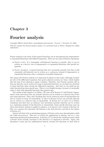
6f(x) AxCHAPTER 3. FOURIER ANALYSISx- L2Figure 4LExample (Sawtooth function): Find the Fourier series for the periodic function shownin Fig. 4. It is defined by f (x) Ax for L/2 x L/2, and it has period L.2Solution: Since f (x) is an odd function of x, only the bn coefficients in Eq. (1) are nonzero.Eq. (12) gives them as2Lbn Z³L/2f (x) sin L/2 22πnxdx LLZ³L/2Ax sin L/2 2πnxdx.L(14)Integrating by parts (or just looking up the integral in a table) gives the general result,Z Z ³x sin(rx) dx11cos(rx) dx cos(rx) dxrrx1 cos(rx) 2 sin(rx).rrx (15)Letting r 2πn/L yields"bn ³ L/2³ L2πn 2 ³ ³L2A2πnx xcos L2πnL L/2 ³ L/22πnx sin L L/2#ALALcos(πn) cos( πn) 02πn2πnAL cos(πn)πnAL.( 1)n 1πn (16)Eq. (1) therefore gives the Fourier trig series for f (x) asf (x) ³ AL X2πnx1( 1)n 1 sinπnL AL2πxsinπLn 1h³ ³ 14πxsin2L ³ 16πxsin3L i ··· .(17)The larger the number of terms that are included in this series, the better the approximationto the periodic Ax function. The partial-series plots for 1, 3, 10, and 50 terms are shownin Fig. 5. We have arbitrarily chosen A and L to be 1. The 50-term plot gives a very goodapproximation to the sawtooth function, although it appears to overshoot the value at thediscontinuity (and it also has some wiggles in it). This overshoot is an inevitable effect at adiscontinuity, known as the Gibbs phenomenon. We’ll talk about this in Section 3.6.Interestingly, if we set x L/4 in Eq. (17), we obtain the cool result,³A·AL11L 1 0 0 ···4π35 π111 1 ···.4357Nice expressions for π like this often pop out of Fourier series.(18)
3.2. FOURIER EXPONENTIAL SERIES7f(x)0.60.6(1 term)(3 .61.01.01.00.20.6(10 terms)0.40.40.20.20.50.51.01.00.5(50 terms)0.50.20.20.40.40.60.61.01.0Figure 53.2Fourier exponential seriesAny function that can be written in terms of sines and cosines can also be written in termsof exponentials. So assuming that we can write any periodic function in the form given inEq. (1), we can also write it as Xf (x) Cn ei2πnx/L(19)f (x)e i2πmx/L dx(20)n where the Cn coefficients are given byCm1 LZL0as we will show below. This hold for all n, including n 0. Eq. (19) is the Fourierexponential series for the function f (x). The sum runs over all the integers here, whereasit runs over only the positive integers in Eq. (1), because the negative integers there giveredundant sines and cosines.We can obtain Eq. (20) in a manner similar to the way we obtained the an and bncoefficients via the orthogonality relations in Eq. (6). The analogous orthogonality relationhere isZ L LL ei2π(n m)x/L ei2πnx/L e i2πmx/L dx i2π(n m)00 0, unless m n,(21)because the value of the exponential is 1 at both limits. If m n, then the integral is simply
8RL0CHAPTER 3. FOURIER ANALYSIS1 · dx L. So in the δnm notation, we have1ZLei2πnx/L e i2πmx/L dx Lδnm .(22)0Just like with the various sine and cosine functions in the previous section, the differentexponential functions are orthogonal.2 Therefore, when we plug the f (x) from Eq. (19) intoEq. (20), the only term that survives from the expansion of f (x) is the one where the nvalue equals m. And in that case the integral is simply Cm L. So dividing the integral by Lgives Cm , as Eq. (20) states. As with a0 in the case of the trig series, Eq. (20) tells us thatC0 L is the area under the curve.Example (Sawtooth function again): Calculate the Cn ’s for the periodic Ax functionin the previous example.Solution: Eq. (20) gives (switching from n to m)Cn The integral of the general formit up in a table). The result isZR1LZL/2Axe i2πnx/L dx.(23) L/2xe rx dx can be found by integration by parts (or lookingx1xe rx dx e rx 2 e rx .rr(24)RThis is valid unless r 0, in which case the integral equals x dx x2 /2. For the specificintegral in Eq. (23) we have r i2πn/L, so we obtain (for n 6 0)Cn ALµ xL i2πnx/L L/2e i2πn L/2³Li2πn 2 L/2 ¶ e i2πnx/L .(25) L/2The second of these terms yields zero because the limits produce equal terms. The first termyields A (L/2)L ¡ iπnCn ·e eiπn .(26)Li2πnThe sum of the exponentials is simply 2( 1)n . So we have (getting the i out of the denominator)iALCn ( 1)n(for n 6 0).(27)2πn L/2If n 0, then the integral yields C0 (A/L)(x2 /2) L/2 0. Basically, the area underthe curve is zero since Ax is an odd function. Putting everything together gives the Fourierexponential series,XiAL i2πnx/Le.(28)f (x) ( 1)n2πnn6 0This sum runs over all the integers (positive and negative) with the exception of 0.1 The “L” in front of the integral in this equation is twice the “L/2” that appears in Eq. (6). This is nosurprise, because if we use eiθ cos θ i sin θ to write the integral in this equation in terms of sines andcosines, we end up with two sin · cos terms that integrate to zero, plus a cos · cos and a sin · sin term, eachof which integrates to (L/2)δnm .2 For complex functions, the inner product is defined to be the integral of the product of the functions,where one of them has been complex conjugated. This complication didn’t arise with the trig functions inEq. (6) because they were real. But this definition is needed here, because without the complex conjugation,the inner product of a function with itself would be zero, which wouldn’t be analogous to regular vectors.
3.2. FOURIER EXPONENTIAL SERIES9As a double check on this, we can write the exponential in terms of sines and cosines:f (x) X( 1)nn6 0³³iAL2πnxcos2πnL ³ i sin2πnxL .(29)Since ( 1)n /n is an odd function of n, and since cos(2πnx/L) is an even function of n, thecosine terms sum to zero. Also, since sin(2πnx/L) is an odd function of n, we can restrictthe sum to the positive integers, and then double the result. Using i2 ( 1)n ( 1)n 1 , weobtain ³ AL X12πnxf (x) ( 1)n 1 sin,(30)πnLn 1in agreement with the result in Eq. (17).Along the lines of this double-check we just performed, another way to calculate theCn ’s that avoids doing the integral in Eq. (20) is to extract them from the trig coefficients,an and bn , if we happen to have already calculated those (which we have, in the case of theperiodic Ax function). Due to the relations,cos z eiz e iz,2andsin z eiz e iz,2i(31)we can replace the trig functions in Eq. (1) with exponentials. We then quickly see that theCn coefficients can be obtained from the an and bn coefficients via (getting the i’s out ofthe denominators)Cn an ibn,2andC n an ibn,2(32)and C0 a0 . The n’s in these relations take on only positive values. For the periodicAx function, we know that the an ’s are zero, and that the bn ’s are given in Eq. (16) as( 1)n 1 AL/πn. So we obtainCn i( 1)n 1AL,2πnandC n i( 1)n 1AL.2πn(33)If we define m to be n in the second expression (so that m runs over the negative integers),and then replace the arbitrary letter m with n, we see that both of these expressions canbe transformed into a single formula,Cn ( 1)niAL,2πn(34)which holds for all integers (positive and negative), except 0. This result agrees with Eq.(27).Conversely, if we’ve already calculated the Cn ’s, and if we want to determine the an ’sand bn ’s in the trig series without doing any integrals, then we can use e z cos z i sin zto write the exponentials in Eq. (19) in terms of sines and cosines. The result will be a trigseries in the form of Eq. (1), with an and bn given byan Cn C n ,andbn i(Cn C n ),(35)and a0 C0 . Of course, we can also obtain these relations by simply inverting the relationsin Eq. (32). We essentially used these relations in the double-check we performed in theexample above.
10CHAPTER 3. FOURIER ANALYSISReal or imaginary, even or oddIf a function f (x) is real (which is generally the case in classical physics), then the nth and( n)th terms in Eq. (19) must be complex conjugates. Because the exponential parts arealready complex conjugates of each other, this implies thatC n Cn (if f (x) is real.(36)For the (real) periodic Ax function we discussed above, the Cn ’s in Eq. (27) do indeedsatisfy C n Cn . In the opposite case where a function is purely imaginary, we must haveC n Cn .Concerning even/odd-ness, a function f (x) is in general neither an even nor an oddfunction of x. But if one of these special cases holds, then we can say something about theCn coefficients. If f (x) is an even function of x, then there are only cosine terms in the trig series inEq. (1), so the relative plus sign in the first equation in Eq. (31) implies thatCn C n .(37)If additionally f (x) is real, then the C n Cn requirement implies that the Cn ’s arepurely real. If f (x) is an odd function of x, then there are only sine terms in the trig series in Eq.(1), so the relative minus sign in the second equation in Eq. (31) implies thatCn C n .(38)This is the case for the Cn ’s we found in Eq. (27). If additionally f (x) is real, thenthe C n Cn requirement implies that the Cn ’s are purely imaginary, which is alsothe case for the Cn ’s in Eq. (27).We’ll talk more about these real/imaginary and even/odd issues when we discuss Fouriertransforms.3.3Fourier transformsThe Fourier trigonometric series given by Eq. (1) and Eqs. (9,11,12), or equivalently theFourier exponential series given by Eqs. (19,20), work for periodic functions. But what if afunction isn’t periodic? Can we still write the function as a series involving trigonometricor exponential terms? It turns out that indeed we can, but the series is now a continuousintegral instead of a discrete sum. Let’s see how this comes about.The key point in deriving the continuous integral is that we can consider a nonperiodicfunction to be a periodic function on the interval L/2 x L/2, with L . Thismight sound like a cheat, but it is a perfectly legitimate thing to do. Given this strategy,we can take advantage of all the results we derived earlier for periodic functions, with theonly remaining task being to see what happens to these results in the L limit. We’llwork with the exponential series here, but we could just as well work with the trigonometricseries.Our starting point will be Eqs. (19) and (20), which we’ll copy here:f (x) Xn Cn ei2πnx/L ,whereCn 1LZL/2 L/2f (x)e i2πnx/L dx,(39)
3.3. FOURIER TRANSFORMS11where we have taken the limits to be L/2 and L/2. Let’s define kn 2πn/L. Thedifference between successive kn values is dkn 2π(dn)/L 2π/L, because dn is simply1. Since we are interested in the L limit, this dkn is very small, so kn is essentially acontinuous variable. In terms of kn , the expression for f (x) in Eq. (39) becomes (where wehave taken the liberty of multiplying by dn 1)f (x) Xn Xn Cn eikn x (dn)µCn eikn x¶Ldkn .2πBut since dkn is very small, this sum is essentially an integral:¶Z µLekn x dknf (x) Cn2π Z C(kn )eikn x dkn ,(40)(41) where C(kn ) (L/2π)Cn . We can use the expression for Cn in Eq. (39) to write C(kn ) as(in the L limit)ZLL 1 C(kn ) Cn ·f (x)e ikn x dx2π2π L Z 1 f (x)e ikn x dx.(42)2π We might as well drop the index n, because if we specify k, there is no need to mention n.We can always find n from k 2πn/L if we want. Eqs. (41) and (42) can then be writtenasZ Z 1ikxf (x) C(k)e dkwhereC(k) f (x)e ikx dx(43)2π C(k) is known as the Fourier transform of f (x), and vice versa. We’ll talk below about howwe can write things in terms of trigonometric functions instead of exponentials. But theterm “Fourier transform” is generally taken to refer to the exponential decomposition of afunction.Similar to the case with Fourier series, the first relation in Eq. (43) tells us that C(k)indicates how much of the function f (x) is made up of eikx . And conversely, the secondrelation in Eq. (43) tells us that f (x) indicates how much of the function C(k) is made up ofe ikx . Of course, except in special cases (see Section 3.5), essentially none of f (x) is madeup of eikx for one particular value of k, because k is a continuous variable, so there is zerochance of having exactly a particular value of k. But the useful thing we can say is that if dkis small, then essentially C(k) dk of the function f (x) is made up of eikx terms in the rangefrom k to k dk. The smaller dk is, the smaller the value of C(k) dk is (but see Section 3.5for an exception to this).Remarks:1. These expressions in Eq. (43) are symmetric except for a minus sign in the exponent (it’s amatter of convention as to which one has the minus sign), and also a 2π. If you want, you2π, by simply replacing C(k) with a B(k)can define things so that eachexpressionhasa1/ function defined by B(k) 2π C(k). In any case, the product of the factors in front of theintegrals must be 1/2π.
12CHAPTER 3. FOURIER ANALYSIS2. With our convention that one expression has a 2π and the other doesn’t, there is an ambiguitywhen we say, “f (x) and C(k) are Fourier transforms of each other.” Better terminology wouldbe to say that C(k) is the Fourier transform of f (x), while f (x) is the “reverse” Fouriertransform of C(k). The “reverse” just depends on where the 2π is. If x measures a positionand k measures a wavenumber, the common convention is the one in Eq. (43). Making both expressions have a “1/ 2π ” in them would lead to less of a need for the word“reverse,” although there would still be a sign convention in the exponents which would haveto be arbitrarily chosen. However, the motivation for having the first equation in Eq. (43)stay the way it is, is that the C(k) there tells us how much of f (x) is made up of eikx , which is a more natural thing to be concerned with than how much of f (x) is made up of eikx / 2π.The latter is analogous to expanding the Fourier series in Eq. (1) in terms of 1/ 2π times thetrig functions, which isn’t the most natural thing to do. The price to pay for the conventionin Eq. (43) is the asymmetry, but that’s the way it goes.3. Note that both expressions in Eq. (43) involve integrals, whereas in the less symmetric Fourierseries results in Eq. (39), one expression involves an integral and one involves a discrete sum.The integral in the first equation in Eq. (43) is analogous to the Fourier-series sum in the firstequation in Eq. (39), but unfortunately this integral doesn’t have a nice concise name like“Fourier series.” The name “Fourier-transform expansion” is probably the most sensible one.At any rate, the Fourier transform itself, C(k), is analogous to the Fourier-series coefficientsCn in Eq. (39). The transform doesn’t refer to the whole integral in the first equation in Eq.(43). Real or imaginary, even or oddAnything that we can do with exponentials we can also do with trigonometric functions.So let’s see what Fourier transforms look like in terms of these. Because cosines and sinesare even and odd functions, respectively, the best way to go about this is to look at theeven/odd-ness of the function at hand. Any function f (x) can be written uniquely as thesum of an even function and an odd function. These even and odd parts (call them fe (x)and fo (x)) are given byfe (x) f (x) f ( x)2andfo (x) f (x) f ( x).2(44)You can quickly verify that these are indeed even and odd functions. And f (x) fe (x) fo (x), as desired.Remark: These functions are unique, for the following reason. Assume that there is another pairof even and odd functions whose sum is f (x). Then they must take the form of fe (x) g(x) andfo (x) g(x) for some functio
Fourier analysis is the study of how general functions can be decomposed into trigonometric or exponential functions with deflnite frequencies. There are two types of Fourier expansions: † Fourier series: If a (reas