WIXLIB

340M. Doepkechild. In this model, parents care about their own consumption c as well asthe number n and utility V of their surviving children.3 The utility function is:c1 rþ bn V :1 rThroughout the paper, it is assumed that r; b; 2 ð0; 1Þ and V 0. Thedeterministic model can be extended to risk-aversion parameters equal to one(log utility) or bigger than one. However, in those cases the utility associatedwith having zero children is negative infinity, so that the choice problemunder uncertainty (where zero surviving children occur with positiveprobability) is not well defined. I therefore concentrate on the case 0 r 1.Let b denote the number of births, and s is the probability of survival foreach child, where 0 s 1. Mortality is deterministic in the sense that s is thefraction of children surviving. Consequently, the number of surviving children is not constrained to be an integer. The full income of a parent isdenoted by w. Since w is taken as given, the distinction between time andgoods costs for children is irrelevant. It is assumed that each birth is associated with a cost of p, and each surviving child entails an additional cost of q.The budget constraint is then c þ pb þ qn w or, after plugging in the survival function n ¼ sb:U ðc; nÞ ¼c þ ðp þ qsÞb w:Income and cost parameters satisfy w 0, p 0, q 0, and p þ q 0. Atleast one of the costs has to be strictly positive; otherwise, the optimal fertilitychoice is infinity. Both consumption and fertility are restricted to benonnegative. The decision problem in the standard version of the BarroBecker model is:Model A: (Barro-Becker with continuous fertility choice)()ðw ðp þ qsÞbÞ1 r þ bðsbÞ V :max1 r0 b w ðpþqsÞI will now consider two further variations of the Barro-Becker frameworkwhich add realism to the benchmark model. The first extension introducesstochastic survival and restricts fertility choice to be an integer. In this model,the realized number of children is uncertain. I assume that for each birth thereis a constant probability of death, implying that the distribution of survivingchildren is Binomial. Apart from the integer restriction and stochasticsurvival, the model is identical to the benchmark. The decision problem isnow given by:Model B: (Stochastic Barro-Becker with discrete fertility choice)(maxb2fN[0g; b w ðpþqÞbXðw pb qnÞ1 rþ bn V1 rn¼0! )b nb ns ð1 sÞ:nThe second extension adds yet more realism by allowing sequential fertilitychoice, while preserving the integer constraint and stochastic survival ofProblem B. In the sequential model, the period is divided into T þ 1subperiods, running from 0 to T . Parents have a fixed income of w in eachsubperiod. The parameter c 2 ð0; 1Þ is the discount factor between periods.

Child mortality and fertility decline341In each period, parents can give birth to a single child. Since children live formultiple periods, the setup allows to distinguish infant and child mortality.Newborn infants survive with probability si until the next period. If the childsurvives, the probability of surviving the second period of life is sy . Once achild has survived for two periods, it will survive until adulthood for sure.4bt 2 f0; 1g denotes the birth decision in period t, yt 2 f0; 1g represents ayoung child (born in the preceding period), and nt is the number of olderchildren (born at least two periods prior) alive in period t. The cost per birthbt is given by p, a young child yt is associated with cost q, and older children ntdo not involve further expenses.5 The budget constraint in period t isct þ pbt þ qyt w.In the sequential model, parents are able to decide on fertility conditional on the survival of older children. Formally, the choice object of theparent is a sequence of decision rules fbt : Ht ! f0; 1ggTt¼0 which map thestate ht at time t into a birth decision. The state at time t is given byht ¼ fnt ; yt g, where nt 0 is the number of children that were born at leasttwo periods ago and survived, and yt 2 f0; 1g denotes whether there is ayoung child that was born in the preceding period. Since there is at mostone birth per period, the maximum number of children is K. The state spaceis therefore Ht ¼ f0; 1; . . . ; Kg f0; 1g.A parent is fecund only until period K, which imposes the additionalconstraint bt ¼ 0 for K t T . This constraint is imposed to provide amotive for ‘‘hoarding’’ of children. If a child dies after period K, it cannot bereplaced. The evolution of the number of children depends on the number ofolder children nt , on whether there is a newborn bt and a young child yt , andon the survival probabilities. Specifically, for a parent that has nt olderchildren today, the probability of having nt þ 1 tomorrow is zero when thereis no young child and sy if a young child exists. Similarly, the probability ofhaving a young child yt in the next period is si if there is a newborn in thisperiod, and zero otherwise. The probabilities over states are therefore definedrecursively as:Ptþ1 ðn; yÞ ¼ Pt ðn; 0Þ ð1 y þ ð2y 1Þbt ðn; 0Þsi Þþ Pt ðn; 1Þ ð1 y þ ð2y 1Þbt ðn; 1Þsi Þ ð1 sy Þþ Pt ðn 1; 1Þ ð1 y þ ð2y 1Þbt ðn 1; 1Þsi Þ sy :ð1ÞFor example, consider the probability of having three old children and oneyoung child in period six (n ¼ 3, y ¼ 1). In this case, (1) reads:P6 ð3; 1Þ ¼ P5 ð3; 0Þ b5 ð3; 0Þsi þ P5 ð3; 1Þ b5 ð3; 1Þsi ð1 sy Þþ P5 ð2; 1Þ b5 ð2; 1Þsi sy :ð2ÞThe state (n ¼ 3, y ¼ 1) can only be reached if in period five there are eitherthree old children, or two old children and a young child. Therefore (2) sumsover the respective probabilities P5 ð3; 0Þ, P5 ð3; 1Þ, and P5 ð2; 1Þ in period five.Also, there has to be a birth in period five, and the infant has to survive, sinceotherwise there would be no young child in period six. Therefore, eachprobability is multiplied by b5 ðn; yÞsi . If the state in period five is f3; 1g, thereare three old children in period six only if the young child dies. Therefore, therespective probability is also multiplied by 1 sy . Finally, if there are only

342M. Doepketwo old children in period five, the young child has to survive if there are to bethree old children in period six. Hence, the last term is multiplied by sy . Theprobability of having n children survive into adulthood is:P ðnÞ ¼ PT ðn; 1Þ ð1 sy Þ þ PT ðn; 0Þ þ PT ðn 1; 1Þ sy :ð3ÞBirth decisions do not enter here, since there are no births in the final periodof adulthood T . The decision problem in the sequential model is:Model C: (Stochastic Barro-Becker with discrete and sequential fertilitychoice)()1 rT XNXXt ðw pbt ðht Þ qyt Þ P t ð ht Þ þ bmaxcn VP ðnÞ ;1 rfbt gTt¼0 t¼0 h 2Hn¼0ttwhere the probabilities over states Pt ðht Þ and surviving children P ðnÞ arefunctions of the birth decisions as defined in (1) and (3) above, and the initialprobabilities are given by P0 ð0; 0Þ ¼ 1 and P0 ðh0 6¼ f0; 0gÞ ¼ 0 (adults startwithout children).Model C is related to the sequential fertility choice models developed bySah (1991) and Wolpin (1997). In Sah’s model, costs accrue only to survivingchildren, there is no limit to fecundity, and children survive for sure once theymake it through the first period. Under the restrictions p ¼ 0, sy ¼ 1, andK ¼ T our model is a special case of Sah’s multi-period setup. Wolpin (1997)analyzes a three-period model (and employs a multi-period version for estimation) which allows for differential survival of infants and children andlimits fecundity to the first two periods. Model C is a special case of Wolpin’smodel under the restrictions T ¼ 2, K ¼ 1, r ¼ 0, and q ¼ 0.A potential limitation of Model C is that we do not allow the household toborrow or lend in order to smooth income over time. This assumption mayhave an impact on the results if there is a lot of curvature in utility. However,the sensitivity analysis carried out in Sect. 5 will show that the main resultsare robust even when utility is close to linear, in which case there is little desirefor consumption smoothing.3. Analytical findingsIn this section, I examine the effect of mortality decline on fertility in the threevariants of the altruistic-parents model from an analytical perspective. As wewill see, clear-cut theoretical results on the mortality-fertility link are onlyavailable for a few special cases of the general model. Section 4 willcomplement the theoretical results derived here with quantitative findingsfrom a calibrated model. All proofs are contained in the appendix.Proposition 1. Let bðsÞ denote the solution to Model A as a function of s. bðsÞhas the following properties: The number of surviving children sbðsÞ is non-decreasing in s. If p ¼ 0 and q 0, fertility bðsÞ is decreasing in s and sbðsÞ is constant. If p 0 and q ¼ 0, fertility bðsÞ is increasing in s.The intuition for these results is simple. Since parents care only about surviving children and there is no uncertainty, the survival probability s affects

Child mortality and fertility decline343choices only through the full cost of a surviving child p s þ q. Raising slowers this cost, and through the substitution effect therefore increases thenumber of surviving children.In the special case where the cost p for each birth is zero, the total cost of asurviving child is independent of s, and consequently parents choose thepreferred number of surviving children irrespective of s. This implies that thetotal number of births declines in inverse proportion to s as the survivalprobability increases.When the cost component specific to surviving children q is zero, the costof a surviving child is inversely proportional to s. The reaction of the numberof births bðsÞ to changes in s now depends on the price elasticity of thedemand for (surviving) children. Given the assumptions 0 1 and0 r 1, this elasticity is bigger than one, so that the total number of birthsrises as the survival probability increases.In summary, we see that in the deterministic model net fertility alwaysrises as the survival probability increases. What happens to the total numberof births depends on which cost component dominates. If a major fraction ofthe total cost of children accrues for every birth, fertility would tend to increase with the survival probability; the opposite holds if children areexpensive only after surviving infancy.I turn to the stochastic models next.Proposition 2. Let bðsÞ denote the solution to Model B as a function of s. Ifp ¼ 0, the optimal choice bðsÞ is non-increasing in s.Proposition 3. Let bt ðht Þðsi Þ denote the solution to Model C as function of theinfant survival probability si at a given state ht . If p ¼ 0 and sy ¼ 1, bt ðht Þðsi Þ isnon-increasing in si .Thus in both stochastic models, we find that if there is no birth-specificcost, the optimal number of births declines as survival rates increase. Theintuition from the deterministic model therefore carries over to the stochasticcase. Only surviving children are costly, and surviving children is all theparents care about. Consequently, parents adjust their fertility to stay close totheir preferred level of fertility. Notice, however, that even if p ¼ 0 in thestochastic model parents are no longer indifferent with regards to s. A highersurvival probability reduces uncertainty about the number of surviving children, which, given risk aversion, increases expected utility.In the sequential model, in the case p ¼ 0 we can also show that age at firstbirth (weakly) increases with the survival probability. There are no clear-cutresults, however, regarding net fertility. If utility is highly concave in n,parents want to avoid a low number of surviving children. If mortality ishigh, this can give rise to a precautionary demand for children or ‘‘hoarding,’’which declines as mortality (and therefore uncertainty) decreases. However,the opposite effect is also possible, since utility is concave in consumption aswell. If parents are very risk averse in terms of consumption, they might wantto avoid the risk of having too many surviving children (and thereby highexpenditures on children), which would lower the number of births whenmortality is high. While these effects apply in principle to both Model B andModel C, the model with sequential fertility choice is in some sense in betweenthe deterministic and the stochastic model. Since choices are spread out overtime, in this case parents have the possibility of replacing children that die

344M. Doepkeearly in the life cycle, leading to less uncertainty over the realized number ofchildren than in Problem B, where all children are born simultaneously.For similar reasons, no general results are available for the case p 0,even if q ¼ 0. In the deterministic model, in this case total fertility bðsÞ increases in s. In the stochastic model, the opposite may be true if the precautionary motive for having children is important. Consider the case of aparent whose primary concern, due to high risk aversion, is to avoid being leftwithout any surviving children. Fertility will be highest when mortality is highas well, since the parent has to rely on a ‘‘law of large numbers.’’ The numberof births would decline if an increased survival probability lowered uncertainty about the number of surviving children.The theoretical analysis identifies two important factors which influencethe child mortality-fertility nexus: the relative cost of dying and survivingchildren, and the degree of risk aversion regarding the number of surviving children. Since both factors depend nontrivially on model parameters, the question whether reductions in child mortality increase ordecrease net fertility is ultimately quantitative in nature.4. Quantitative findingsThe analytical results show that all three models are consistent with decliningtotal fertility rates (i.e., number of births) in response to falling mortality.However, we are left without a clear-cut prediction for the relationship of childmortality to net fertility (i.e., number of survivors). Only the deterministicmodel unambiguously predicts that the number of surviving children will riseas mortality falls. In the more elaborate stochastic models, the relationshipcould go either way. Therefore, I assess the quantitative predictions of themodels with a calibration exercise. Each model is parameterized to reproducemortality and fertility rates in England in 1861, when infant and childmortality was still high. I then increase the survival parameters to correspondto mortality rates in 1951 (by which time most of the fall in infant and childmortality had been completed) and compare the predictions of each model forthe impact on fertility rates.The models are parameterized as follows. In the sequential model, we setT ¼ 14 and K ¼ 12, so that the maximum number of births is 13. Income w isa scale parameter and is set to 1 per period in the sequential model and 14 inthe other models. The parameter p corresponds to the cost of a child until itsfirst birthday, while the parameter q accounts for the remaining cost. In termsof goods, it is natural to assume that the yearly cost increases until the child isable to work and partly pay for itself. The time cost, on the other hand,decreases over time. In addition, the cost per birth should account for the costof pregnancy and the risk of the mother’s death during childbirth. Since timeand goods cost move in opposite directions, I assume as the baseline case thatoverall cost is proportional to age, and that children are no longer a netburden once they are six years old. I therefore set q p ¼ 5. The overall level ofthe cost parameters is set such that in the sequential model, a household withboth an infant and a young child spends half of its income on the children.This gives p ¼ 1 12 and q ¼ 5 12. The curvature parameters in the utilityfunction are set to r ¼ ¼ 1 2, and the discount factor in the sequentialmodel is c ¼ 0:95. The children’s utility level V is equated to the parent’s

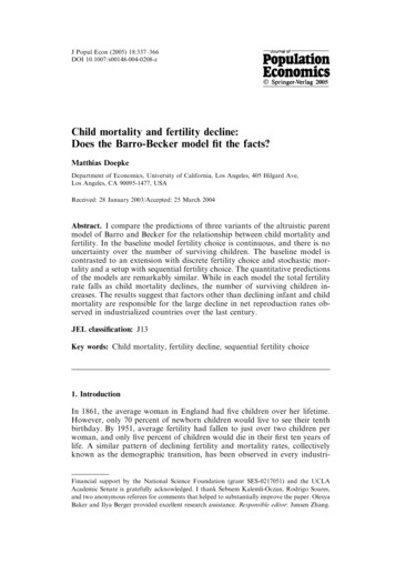
Child mortality and fertility decline345utility in each case (i.e., the steady-state utility that would obtain with constant income and mortality rates).The survival parameters are chosen to correspond to the situation inEngland in 1861. According to Perston et al. (1972) the infant mortality rate(death rate until first birthday) was 16%, while the child mortality rate(death rate between first and fifth birthday) was 13%. Accordingly, I setsi ¼ 0:84 and sy ¼ 0:87 in the sequential model, and s ¼ si sy ¼ 0:73 in theother models. Finally, the altruism factor b is set in each model to match thetotal fertility rate, which was 4.9 in 1861 (Chenais 1992). Since fertilitychoice is discrete in Models B and C, I chose a total fertility rate of 5.0 asthe target.Each model is thus calibrated to reproduce the relationship of fertility andinfant and child mortality in 1861. I now examine how fertility adjusts whenmortality rates fall to the level observed in 1951, which is 3% for infantmortality and 0.5% for child mortality. The results for fertility can be compared to the observed total fertility rate of 2.1 in 1951.In Model A (Barro-Becker with continuous fertility choice), the totalfertility rate falls from 5.0 (the calibrated target) to 4.2 when mortality ratesare lowered to the 1951 level. The expected number of surviving childrenincreases from 3.7 to 4.0. Thus, there is a small decline in total fertility, but (aswas to be expected given Proposition 1) an increase in the net fertility rate.Perhaps surprisingly, the results generated by Model B (stochastic BarroBecker with discrete fertility choice) are very similar to Model A. In thestochastic model, total fertility falls from 5.0 to 4.0, and net fertility increasesfrom 3.7 to 3.9. Fertility falls by more than in the deterministic model, but thedifference is small.In Model C (sequential fertility choice), the total fertility rate is not aninteger since it depends on the random individual mortality realizations.Therefore, b was chosen to move the total fertility rate to 5.2, which is theclosest possible match to the target of 5.0. When mortality is lowered to 1951levels, fertility falls only to 5.0, while net fertility increases substantially from3.8 to 4.8. These results are partly due to the fact that the sequential modeldistinguishes infant and child mortality, while the other models do not. Thesequential model probably overstates the cost of child mortality, since weassume that the entire cost q has to be paid if a child dies, even though mostof child mortality is concentrated near the beginning of the interval from oneto five years of age. The models line up more closely if we set sy ¼ 1 andassign the entire fall in mortality to infant mortality si (as we do implicitly inthe other two models). In this case, total fertility falls from 5.1 to 4.0, whilenet fertility increases from 3.7 to 3.9. This is identical to the results withModel B.Figures 1 to 3 show that the predictions of the models are similar for theentire range of possible infant mortality rates (the solid line is the total fertility rate, and the dotted line is the net fertility rate; for Fig. 3, child mortalitywas set to sy ¼ 1). The sequential model yields additional predictions for theage at first birth, which increases with the survival probability once si is atleast 10 percent (Fig. 4). This increase not only reflects the correspondingdecline in total fertility, but also narrower spacing of births. When mortalityis high, parents start having children early so that there is time to make up forchildren who die. This replacement motive is less important when survivalrates are high.

346M. DoepkeFig. 1. Births and survivors in the benchmark modelFig. 2. Births and survivors in the binomial modelFig. 3. Births and survivors in the sequential modelIn terms of guiding the applied researcher, our results show that once thedifferential cost of dying and surviving children is accounted for, the deterministic Barro-Becker model leads to virtually the same conclusions as the

Child mortality and fertility decline347Fig. 4. Age at first birth in the sequential modelstochastic model with sequential fertility choice. Thus, unless questionsconcerning birth order and timing are of particular interest (as in Caucutt et al.2002), the basic model can be used as a stand-in for the more elaborate setup.In all computations, the children’s utility V was held constant. However,results are virtually unchanged if V is adjusted to reflect the steady-stateutility at each value of s. This utility increases in s since the cost of survivingchildren falls as s increases, while uncerta

insurance mechanism against the future death of some of their children. A decline in child mortality will translate into a decline in net fertility only if the hoarding motive is sufficiently strong. We will see that, theoretically, such a response can indeed arise if it is impossible to replace dying children, and if