Transcription
Discovery of Spatial Association Rules? inGeographic Information DatabasesKrzysztof Koperski and Jiawei HanSchool of Computing ScienceSimon Fraser UniversityBurnaby, B.C., Canada V5A 1S6e-mail: fkoperski, hang@cs.sfu.caAbstract. Spatial data mining, i.e., discovery of interesting, implicitknowledge in spatial databases, is an important task for understandingand use of spatial data- and knowledge-bases. In this paper, an e cientmethod for mining strong spatial association rules in geographic information databases is proposed and studied. A spatial association rule is arule indicating certain association relationship among a set of spatial andpossibly some nonspatial predicates. A strong rule indicates that the patterns in the rule have relatively frequent occurrences in the database andstrong implication relationships. Several optimization techniques are explored, including a two-step spatial computation technique (approximatecomputation on large sets, and re ned computations on small promisingpatterns), shared processing in the derivation of large predicates at multiple concept levels, etc. Our analysis shows that interesting associationrules can be discovered e ciently in large spatial databases.1 IntroductionWith wide applications of remote sensing technology and automatic data collection tools, tremendous amounts of spatial and nonspatial data have beencollected and stored in large spatial databases. Traditional data organizationand retrieval tools can only handle the storage and retrieval of explicitly storeddata. The extraction and comprehension of the knowledge implied by the hugeamount of spatial data, though highly desirable, pose great challenges to currently available spatial database technologies.This situation demands new technologies for knowledge discovery in large spatial databases, or spatial data mining, that is, extraction of implicit knowledge,spatial relations, or other patterns not explicitly stored in spatial databases.Recently, there have been a lot of research activities on knowledge discoveryin large databases (data mining) 9, 16]. These studies led to a set of interesting techniques developed, including mining strong association and dependency?This research was supported in part by the research grant NSERC-OGP003723 fromthe Natural Sciences and Engineering Research Council of Canada and an NCE/IRISresearch grant from the Networks of Centres of Excellence of Canada.
rules 1, 2], attribute-oriented induction for mining characteristic and discriminant rules 12], etc. Such studies set a foundation and provide some interestingmethods for the exploration of highly promising spatial data mining techniques.Spatial data mining can be categorized based on the kinds of rules to bediscovered in spatial databases. A spatial characteristic rule is a general description of a set of spatial-related data. For example, the description of the generalweather patterns in a set of geographic regions is a spatial characteristic rule.A spatial discriminant rule is the general description of the contrasting or discriminating features of a class of spatial-related data from other class(es). Forexample, the comparison of the weather patterns in two geographic regions isa spatial discriminant rule. A spatial association rule is a rule which describesthe implication of one or a set of features by another set of features in spatialdatabases. For example, a rule like \most big cities in Canada are close to theCanada-U.S. border" is a spatial association rule.There have been some interesting studies related to the mining of spatialcharacteristic rules and spatial discriminant rules 14, 15]. However, there islack of studies on mining spatial association rules. In this paper, we study theextension of the techniques for mining association rules in transaction-baseddatabases to mining spatial association rules.A spatial association rule is a rule of the form \X ! Y ", where X and Y aresets of predicates and some of which are spatial ones. In a large database manyassociation relationships may exist but some may occur rarely or may not holdin most cases. To focus our study to the patterns which are relatively strong,i.e., which occur frequently and hold in most cases, the concepts of minimumsupport and minimum con dence are introduced 1, 2]. Informally, the supportof a pattern A in a set of spatial objects S is the probability that a member of Ssatis es pattern A and the con dence of A ! B is the probability that patternB occurs if pattern A occurs. A user or an expert may specify thresholds tocon ne the rules to be discovered to be strong ones.For example, one may nd that 92% of cities within British Columbia (bc)and adjacent to water are close to U.S.A., as shown in (1), which associatespredicates is a, within, and adjacent to with spatial predicate close to.is a(X city) within(X bc) adjacent to(X water) ! close to(X us): (92%)(1)Although such rules are usually not 100% true, they carry some nontrivialknowledge about spatial associations, and thus it is interesting to \mine" (i.e.,\discover") them from large spatial databases. The discovered rules will be usefulin geography, environmental studies, biology, engineering and other elds.In this paper, e cient methods for mining spatial association rules are studied, with a top-down, progressive deepening search technique proposed. Thetechnique rstly searches at a high concept level for large (i.e., frequently occurring) patterns and strong implication relationships among the large patternsat a coarse resolution scale. Then only for those large patterns, it deepens thesearch to lower concept levels (i.e., their lower level descendants). Such a deepening search process continues until no large patterns can be found. An important
optimization technique is that the search for large patterns at high concept levels may apply e cient spatial computation algorithms at a coarse resolutionscale (such as generalized close to (g close to), using approximate spatial computation algorithms, such as R-trees or plane-sweep techniques operating onminimum bounding rectangles (MBRs). Only the candidate spatial predicates,which are worth detailed examination, will be computed by re ned spatial techniques(giving detailed predicates such as intersect, contain, etc.). Such multiplelevel approach saves much computations because it is very expensive to performdetailed spatial computation for all the possible spatial association relationships.In Sect. 2 of our paper, existing spatial data mining methods are surveyed. InSect. 3, the concept of spatial association rules and its data mining methods areoutlined. In Sect. 4, an algorithm for the discovery of spatial association rules ispresented. In Sect. 5 we discuss the advantages of the algorithm and its possibleextensions. The study is summarized in Sect. 6.2 Previous Work Related to Spatial Data MiningIn this section, previous studies related to spatial data mining are overviewed,which provides a short survey of the topic and associates the previous work withour study.2.1 Statistical AnalysisUntil now statistical spatial analysis has been one of the most common techniques for analyzing spatial data 10]. Statistical methods handle well numericaldata, contain a large number of algorithms, have a strong possibility of getting models of spatial phenomena, and allow optimizations. However, statisticalanalysis usually requires the assumptions regarding to statistical independenceof spatially distributed data. Such assumptions are often unrealistic due to thein uence of neighboring regions. To deal with such problems, spatial models caninclude trend surface or dummy variables. If data in one region are in uencedby features of neighboring regions, the analyst may t a regression model witha spatial lagged forms of the dependent variables. Statistical analysis also dealspoorly with symbolic data like names.expensive(condo) inside(condo downtown) area(condo large):(2)Nonlinear rules in the form of (2) cannot be described using standard methodsin statistical spatial analysis. Statistical approach requires a lot of domain andstatistical knowledge. Thus, it should be performed by domain experts with theexperience in statistics. Another problem related to statistical spatial analysis isexpensive computation of the results.2.2 Generalization-based Spatial Data MiningOne major approach in spatial data mining is to apply generalization techniquesto spatial and nonspatial data to generalize detailed spatial data to certain highlevel and study the general characteristics and data distributions at this level.
An attribute-oriented induction method has been proposed in 14]. It generalizes data to high level concepts and describes general relationships betweenspatial and nonspatial data. Two algorithms were proposed in the study: (1)nonspatial-dominant generalization, and (2) spatial-dominant generalization.The nonspatial-dominant generalization algorithm rst performs attributeoriented generalization on task-relevant nonspatial data describing the propertiesof spatial objects. In this step, numerical data can be generalized to ranges ordescriptive high level concepts (e.g., ;9 C to a range value \;10 to 0 C" orcold), and symbolic values to higher level concepts (e.g., potatoes and beets tovegetables). By doing so, low level distinctive values may be generalized to identical high level values, and such high-level identical values among di erent tuplescan be merged together with their spatial pointers clustered into one slot in thespatial attribute. Finally, the map consists of a small number of regions withhigh level descriptions.The spatial-dominant generalization rst performs generalization on queryrelated spatial data. Data are generalized using spatial data hierarchies (such asgeographic or administrative regions) provided by users/experts or hierarchicaldata structures (such as quad-trees 19] or R-trees 11]). The generalized spatialentities (such as the merged regions) cluster the related nonspatial data together.After generalization of non-spatial data, every region can be described at a highconcept level by one or a set of predicates.Spatial hierarchies are not always given a priori. It is often necessary todescribe spatial behavior of similar objects or to determine characteristic features of distinct clusters. In 15], the attribute-oriented induction method wascombined with some e cient spatial clustering algorithms, which can still beclassi ed into spatial-dominant vs. nonspatial-dominant methods. The spatialdominant method classi es task-relevant spatial objects (such as points) intoclusters using an e cient clustering algorithm and then perform an attributeoriented induction for each cluster to extract rules describing general propertiesof a cluster. The nonspatial-dominant method rst generalizes nonspatial attributes of query-related objects to high concept levels and then cluster thespatial objects with the same nonspatial descriptions. Then one may nd that\expensive single houses in Vancouver area are clustered along the beach andaround two city parks".2.3 Other Relevant StudiesAlso knowledge mining in image databases, which can be treated as a specialtype of spatial databases, has been studied recently. Method for the classi cationof sky objects and another method for recogntion of volcanos on the surface ofVenus are described in 8], where classi cation trees were used to make naldecisions.Sky objects were classi ed as stars or galaxies. In the rst step of the algorithm, basic attributes describing each object were extracted. Attributes likearea, sky brightness, positions of peak brightness, and intensity image moments,
etc. were produced. The training set was classi ed by astronomers, and attributesmentioned above were used to construct the decision tree.In the study of volcanos attributes recognized by humans like diameters andcentral peaks are not su cient for the classi cation. Thus, eigenvalues of matrices representing images of possible volcanos were used as attributes for theclassi cation algorithm.The studies on data mining in relational databases 1, 2, 12, 13, 16] areclosely related to spatial data mining. In particular, the previous studies onmining association rules 1, 2, 13] are closely related to this study.An association rule is a general form of dependency rule and is de ned ontransaction-based databases 1]. It is in the form of \W ! B (c%)", explainedas, \if a pattern W appears in a transaction, there is c% possibility (con dence)that the pattern B holds in the same transaction", where W and B are a set ofattribute values. Moreover, to ensure that such rules are interesting enough tocover frequently encountered patterns in a database, the concept of the supportof a rule \W ! B" is introduced, which is de ned as the ratio that the patterns of W and B occurring together in the transactions vs. the total number oftransactions in the database. For example, in a shopping transaction databaseone may nd a rule like \butter ! bread (90%)", which means that 90% of customers who buy butter also purchase bread. E cient algorithms for the discoveryof such kind of rules in transaction-based databases have been studied 1, 2].3 Spatial Association RulesGeneralization-based spatial data mining methods 14, 15] discover spatial andnonspatial relationships at a general concept level, where spatial objects are expressed as merged spatial regions 14] or clustered spatial points 15]. However,these methods cannot discover rules re ecting structure of spatial objects andspatial/spatial or spatial/nonspatial relationships which contain spatial predicates, such as adjacent to, near by, inside, close to, intersecting, etc.As a complementary, spatial association rules represents object/predicaterelationships containing spatial predicates. For example, the following rules arespatial association rules.{ Nonspatial consequent with spatial antecedent(s).is a(x house) close to(x beach) ! is expensive(x): (90%){ Spatial consequent with non-spatial/spatial antecedent(s).is a(x gas station) ! close to(x highway): (75%)Various kinds of spatial predicates can be involved in spatial association rules.They may represent topological relationships 6] between spatial objects, suchas disjoint, intersects, inside/outside, adjacent to, covers/covered by, equal, etc.They may also represent spatial orientation or ordering, such as left, right, north,east, etc., or contain some distance information, such as close to, far away, etc.
For systematic study the mining of spatial association rules, we rst introducesome preliminary concepts.De nition1. A spatial association rule is a rule in the form ofP1 : : : Pm ! Q1 : : : Qn: (c%)(3)where at least one of the predicates P1 : : : Pm Q1 : : : Qn is a spatial predicate,and c% is the con dence of the rule which indicates that c% of objects satisfyingthe antecedent of the rule will also satisfy the consequent of the rule.2Following this de nition, a large number of spatial association rules can bederived from a large spatial database. However, most people will be only interested in the patterns which occur relatively frequently (i.e., with large supports)and the rules which have strong implications (i.e., with high con dence). Therules with large supports and high con dence are strong rules.De nition2. The support of a conjunction of predicates, P P1 : : : Pk,in a set S, denoted as (P S), is the number of objects in S which satisfy Pversus the cardinality (i.e., the total number of objects) of S. The con denceof a rule P ! Q in S, '(P ! Q S), is the ratio of (P Q S) versus (P S),i.e., the possibility that Q is satis ed by a member of S when P is satis ed bythe same member of S. A single predicate is called 1-predicate. A conjunctionof k single predicates is called a k-predicate.2Since most people are interested in rules with large supports and high con dence, two kinds of thresholds: minimum support and minimum con dence, canbe introduced. Moreover, since many predicates and concepts may have strongassociation relationships at a relatively high concept level, the thresholds shouldbe de ned at di erent concept levels. For example, it is di cult to nd regularassociation patterns between a particular house and a particular beach, however,there may be strong associations between many expensive houses and luxurious beaches. Therefore, it is expected that many spatial association rules areexpressed at a relatively high concept level.De nition3. A set of predicates P is large in set S at level k if the support ofP is no less than its minimum support threshold k0 for level k, and all ancestorsof P from the concept hierarchy are large at their corresponding levels. Thecon dence of a rule \P ! Q S" is high at level k if its con dence is no lessthan its corresponding minimum con dence threshold '0k .2De nition4. A rule \P ! Q S" is strong if predicate \P Q" is large in setS and the con dence of \P ! Q S" is high.2Based on these de nitions, an example is presented for the explanation of theprocess of mining strong spatial association rules in large databases. To facilitatethe speci cation of the primitives for spatial data mining, an SQL-like spatialdata mining query interface, which is designed based on a spatial SQL proposedin 7], has been speci ed for an experimental spatial data mining system prototype, GeoMiner, which is currently under implementation and experimentation.
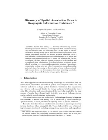
Example 1. Let the spatial database to be studied adopt an extended-relationaldata model and a SAND (spatial-and-nonspatial database) architecture 3]. Thatis, it consists of a set of spatial objects and a relational database describingnonspatial properties of these objects.Our study of spatial association relationships is con ned to British Columbia,a province in Canada, whose map is presented in Fig. 1, with the followingdatabase relations for organizing and representing spatial objects.1. town(name type population geo : : :).2. road(name type geo : : :).3. water(name type geo : : :).4. mine(name type geo : : :).5. boundary(name type admin region 1 admin region 2 geo : : :).Notice that in the above relational schemata, the attribute \geo" represents aspatial object (a point, line, area, etc.) whose spatial pointer is stored in a tupleof the relation and points to a geographic map. The attribute \type" of a relationis used to categorize the types of spatial objects in the relation. For example, thetypes for road could be fnational highway, local highway, street, back laneg, andthe types for water could be focean, sea, inlets, lakes, rivers, bay, creeksg. Theboundary relation speci es the boundary between two administrative regions,such as B.C. and U.S.A. (or Alberta). The omitted elds may contain otherpieces of information, such as the area of a lake and the ow of a river.Suppose a user is interested in nding within the map of British Columbia thestrong spatial association relationships between large towns and other \near by"objects including mines, country boundary, water (sea, lake, or river) and majorhighways. The GeoMiner query is presented below.discover spatial association rulesinside British Columbiafrom road R, water W, mines M, boundary Bin relevance to town Twhere g close to(T.geo, X.geo) and X in fR, W, M, Bgand T.type large'' and R.type in fdivided highwaygand W.type in fsea, ocean, large lake, large rivergand B.admin region 1 in B.C.''and B.admin region 2 in U.S.A.''Notice that in the query, a relational variable X is used to represent one ofa set of four variables fR, W, M, Bg, a predicate close to(A, B) says that aspatial objects A and B are close one to another, and g close to is a prede ned generalized predicate which covers a set of spatial predicates: intersect,adjacent to, contains, close to.Moreover, \close to" is a condition-dependent predicate and is de ned by aset of knowledge rules. For example, a rule in (4) states if X is a town and Y isa country, then X is close to Y if their distance is within 80 kms.
large cityminelarge riverdivided highwaylakeFig.1. The map of BC.close to(X Y ) is a(X town) is a(Y country) dist(X Y d) d 80 km:(4)close to(X Y ) is a(X town) is a(Y road) dist(X Y d) d 5 km: (5)However, \close to" between a town and a road will be de ned by a smallerdistance such as (5).Furthermore, we assume in the B.C. map, admin region 1 always contains aregion in B.C., and thus \U.S.A." or its states must be in \B.admin region 2".Since there is no constraint on the relation \mine", it essentially means, \M.typein ANY", which is thus omitted in the query.To facilitate mining multiple-level association rules and e cient processing,concept hierarchies are provided for both data and spatial predicates.A set of hierarchies for data relations are de ned as follows.{ A concept hierarchy for towns:(town (large town (big city, medium sized city), small town (: : :) : : :) : : :).{ A concept hierarchy for water:(water (sea (strait (Georgia Strait, : : :), Inlet (: : : ), : : :),river (large river (Fraser River, : : :), : : :),lake (large lake (Okanagan Lake, : : :), : : :), : : : ), : : :){ A concept hierarchy for road:(road (national highway (route1, : : :),provincial highway (highway 7, : : :),city drive (Hasting St., Kingsway, : : :),city street (E 1st Ave., : : :), : : :), : : :)Spatial predicates (topological relations) should also be arranged into a hierarchy for computation of approximate spatial relations (like \g close to" in Fig.
g close tonot disjointINTERSECTSadjacent to intersectsINSIDEcovered byclose toCONTAINSinsidecoversEQUALcontainsFig. 2. The hierarchy of topological relations.2) using e cient algorithms with coarse resolution at a high concept level andre ne the computation when it is con ned to a set of more focused candidateobjects.24 A Method for Mining Spatial Association Rules4.1 An Example of Mining Spatial Association RulesExample 2. We examine how the data mining query posed in Example 1 is pro-cessed, which illustrates the method for mining spatial association rules.Firstly, the set of relevant data is retrieved by execution of the data retrievalmethods 3] of the data mining query, which extracts the following data setswhose spatial portion is inside B.C.: (1) towns: only large towns (2) roads: onlydivided highways2 (3) water: only seas, oceans, large lakes and large rivers (4)mines: any mines and (5) boundary: only the boundary of B.C., and U.S.A.Secondly, the \generalized close to" (g close to) relationship between (large)towns and the other four classes of entities is computed at a relatively coarseresolution level using a less expensive spatial algorithm such as the MBR datastructure and a plane sweeping algorithm 18], or R*-trees and other approximations 5]. The derived spatial predicates are collected in a \g close to" table(Table 1), which follows an extended relational model: each slot of the table maycontain a set of entries. The support of each entry is then computed and thosewhose support is below the minimum support threshold, such as the column\mine", are removed from the table.Notice that from the computed g close to relation, interesting large item setscan be discovered at di erent concept levels and the spatial association rulescan be presented accordingly. For example, the following two spatial associationrules can be discovered from this relation.is a(X large town) ! g close to(X water): (80%)is a(X large town) g close to(X sea) ! g close to(X us boundary):(92%)2Not all the segments of national and provincial highways in Canada are divided ones,our computation only counts the divided ones. Also, \provincial divided highway" isabbreviated to \provincial highway" in later presentations.
TownWaterRoadBoundary MineVictoria Juan de Fuca Strait highway 1, highway 17 USSaanich Juan de Fuca Strait highway 1, highway 17 USPrince Georgehighway 97PentinctonOkanagan Lakehighway 97US Alalla:::::::::::::::Table 1. The computed \g close to" relation.The detailed computation process is not presented here since it is similar tomining association rules for exact spatial relationships to be presented below.Since many people may not be satis ed with approximate spatial relationships, such as g close to, more detailed spatial computation often needs to beperformed to nd the re ned (or precise) spatial relationships in the spatialpredicate hierarchy. Thus we have the following steps.Re ned computation is performed on the large predicate sets, i.e., thoseretained in the g close to table. Each g close to predicate is replaced by one ora set of concrete predicate(s) such as intersect, adjacent to, close to, inside, etc.Such a process results in Table 1i,hadjacent to, J.Fuca Straiti hintersects, highway 17i hclose to, USihighway 1i,Saanichhadjacent to, J.Fuca Straiti hhintersects,close to, highway 17i hclose to, USiPrince Georgehintersects, highway 97iPentincton hadjacent to, Okanagan Lakei hintersects, highway 97i hclose to, USi::::::::::::Table 2. Detailed spatial relationships for large sets.Table 2 forms a base for the computation of detailed spatial relationships atmultiple concept levels. The level-by-level detailed computation of large predicates and the corresponding association rules is presented as follows.The computation starts at the top-most concept level and computes largepredicates at this level. For example, for each row of Table 2 (i.e., each largetown), if the water attribute is nonempty, the count of water is incremented byone. Such a count accumulation forms 1-predicate rows (with k 1) of Table3 where the support count registered. If the (support) count of a row is smallerthan the minimum support threshold, the row is removed from the table. Forexample, the minimum support is set to 50% at level 1, a row whose countis less than 20, if any, is removed from the table. The 2-predicate rows (i.e.,
k 2) are formed by the pair-wise combination of the large 1-predicates, withtheir count accumulated (by checking against Table 2). The rows with the countsmaller than the minimum support will be removed. Similarly, the 3-predicatesare computed. Thus, the computation of large k-predicates results in Table 3.klarge k-predicate setcount1 hadjacent to, wateri321 hintersects, highwayi291 hclose to, highwayi291 hclose to, us boundaryi282 hadjacent to, wateri, hintersects, highwayi252 hadjacent to, wateri, hclose to, us boundaryi232 hclose to, us boundaryi , hintersects, highwayi263 hadjacent to, wateri, hclose to, us boundaryi , hintersects, highwayi 22Table 3. Large k-predicate sets at the top concept level (for 40 large towns in B.C.).Spatial association rules can be extracted directly from Table 3. For example,to, wateri,since hintersects, highwayi has a support count of 29, and hadjacenthintersects, highwayi has a support count of 25, and 25 29 : 86%, we have theassociation rule (6).is a(X large town) intersects(X highway) ! adjacent to(X water): (86%)(6)Notice that a predicate \is a(X large town)" is added in the antecedent of therule since the rule is related only to large town.Similarly, one may derive another rule (7). However, if the minimum con dence threshold were set to 75%, this rule (with only 72% con dence) wouldhave been removed from the list of the association rules to be generated.is a(X large town) adjacent to(X water) ! close to(X us boundary):(72%)(7)After mining rules at the highest level of the concept hierarchy, large kpredicates can be computed in the same way at the lower concept levels, whichresults in Tables 4 and 5. Notice that at the lower levels, usually the minimumsupport and possibly the minimum con dence may need to be reduced in orderto derive enough interesting rules. For example, the minimum support of level2 is set to 25% and thus the row with support count of 10 is included in Table4 whereas the minimum support of level 3 is set to 15% and thus the row withsupport count of 7 is included in Table 5.Similarly, spatial association rules can be derived directly from the large kpredicate set tables at levels 2 and 3. For example, rule (8) is found at level 2,and rule (9) is found at level 3.is a(X large town) ! adjacent to(X sea) (52:5%) (8)is a(X large town) adjacent to(X georgia strait) ! close to(X us):(78%) (9)
klarge k-predicate setcount1 hadjacent to, seai211 hadjacent to, large riveri111 hclose to, us boundaryi281 hintersects, provincial highwayi211 hclose to, provincial highwayi242 hadjacent to, seai, hclose to, us boundaryi152 hclose to, us boundaryi , hintersects, provincial highwayi192 hadjacent to, seai, hclose to, provincial highwayi112 hclose to, us boundaryi , hclose to, provincial highwayi223 hadjacent to, seai, hclose to, us boundaryi , hclose to, provincial highwayi 10Table 4. Large k-predicate sets at the second level (for 40 large towns in B.C.).klarge k-predicate setcount1 hadjacent to, georgia straiti91 hadjacent to, fraser riveri101 hclose to, us boundaryi282 hadjacent to, georgia straiti, hclose to, us boundaryi 7Table 5. Large k-predicate sets at the third level (for 40 large towns in B.C.).Notice that only the descendants of the large 1-predicates will be examinedat a lower concept level. For example, the number of large towns adjacent toa lake is small and thus hadjacent to, lakei is not represented in Table 4. Thenthe predicates like hadjacent to okanagan lakei will not be even considered atthe third level. The mining process stops at the lowest level of the hierarchies orwhen an empty large 1-predicate set is derived.As an alternative of the problem, large towns may also be further partitioned into big cities (such as towns with a population larger than 50,000 people), other large towns, etc. and rules like rule (10) can b
An attributeorien ted induction metho d has b een prop osed in It gen eralizes data to high lev el concepts and describ es general relationships b et