Transcription
DATA VISUALIZATION THROUGHGRAPH DRAWINGGEORGE MICHAILIDIS AND JAN DE LEEUWAbstract. In this paper the problem of visualizing data sets is considered.By representing the data as the adjacency matrix of an appropriately definedbipartite graph, the problem is transformed to one of graph drawing. A general graph drawing framework is introduced, the corresponding mathematicalproblem defined and an algorithmic approach for solving the necessary optimization problem discussed. The new approach is illustrated through severalexamples.1. IntroductionAdvances in data collection, computerization of transactions and breakthroughsin storage technology have allowed research and business organizations to collectincreasingly large amounts of data. In order to extract useful information fromsuch large data sets, a first step is to be able to visualize their global structure andidentify patterns, trends and outliers.Graphs are useful entities since they can represent relationships between setsof objects. They are used to model complex systems (e.g. computer and transportation networks, VLSI and Web site layouts, molecules, etc) and to visualizerelationships (e.g. social networks, entity-relationship diagrams in database systems, etc). Graphs are also very interesting mathematical objects and a lot ofattention has been paid to their properties. In many instances the right picture isthe key to understanding. The various ways of visualizing a graph provide differentinsights, and often hidden relationships and interesting patterns are revealed. Anincreasing body of literature is considering the problem of how to draw a graph(see for instance the book by [6] on Graph Drawing, the proceedings of the annualconference on Graph Drawing, etc). Also, several problems in distance geometryand in graph theory have their origin in the problem of graph drawing in higher dimensional spaces. Of particular interest are the representation of data sets throughgraphs. This bridges the fields of multivariate statistics and graph drawing.Despite the recent explosive growth of the graph drawing field, the various techniques proposed exhibit a high degree of arbitrariness, and more often than not lacka rigorous mathematical background. In this paper, we provide a rigorous mathematical framework of drawing graphs utilizing the information contained in theadjacency matrix of the underlying graph. At the core of our approach are variousloss functions that measure the lack of fit of the resulting representation, that needto be optimized subject to a set of constraints that correspond to different drawing1
2GEORGE MICHAILIDIS AND JAN DE LEEUWrepresentations. We then establish how the graph drawing problem encompassesproblems in multivariate statistics. We develop a set of algorithms based on thetheory of majorization to optimize the various loss functions and study their properties (existence of solution, convergence, etc). We demonstrate the usefulness ofour approach through a series of examples.2. Data as Graphs2.1. Graphs and the Adjacency Matrix. In this paper we consider an undirected graph G (V, E), where V {v1 , v2 , . . . , vn } is the set of the n vertices andE V V the set of edges. It is assumed that the graph G does not contain eitherself-loops or multiple edges between any pair of vertices. The set of edges can berepresented in matrix form through the adjacency matrix A {aij , i, j 1, . . . , n}.Thus, vertices i, j G are connected if and only if aij 0, otherwise aij 0. Ifaij {0, 1} we are dealing with a simple graph, otherwise a weighted graph.In the following example the graph representation of a familiar data structurefrom multivariate statistics is given. Consider the following dissimilarity matrix 0 7 0 2 3 0 8 6 1 0 5 9 6 3 0 3 1 2 5 12 0It can be represented by a complete weighted graph on 6 vertices as shown in Figure1. #"!#! 3 #"!#! ## ## #"! #"! #"! !#!#!# """ " " # 7 #"! #! #"!#! #"!#! #"!#! #"!#! ## " " " " " 5 # # !#!#!# !##"#! " """ " ! " ! " ! 8"! ! " ! " !! 2 ! ! ! ! ! ! " " "" ! " " " " " Figure 1. The graph representation of a dissimilarity matrix2.2. Bipartite Graphs. In two recent papers of de Leeuw and Michailidis [5,13] the problem of representing categorical datasets through bipartite graphs isconsidered. For bipartite graphs, the vertex set V is partitioned into two sets V1and V2 , and the edge set E is defined on V1 V2 and indicates which vertices from V1are connected to vertices in V2 and vice versa. In multidimensional data analysis,the classical data structure where data on J categorical variables (with kj possiblevalues (categories) per variable) are collected for N objects, can be representedP bya bipartite graph. The N objects correspond to the vertices of V1 , the K j kjcategories to the vertices of V2 and there are N J edges in E, since each objectis connected to J different categories.
DATA VISUALIZATION3The adjacency matrix of a bipartite graph takes the form 0 WA W0 0Sleeping BagPriceOne Kilo BagSundKompakt BasicFinmark TourInterlight LyxKompaktTouch the CloudCat’s MeowIgloo SuperDonnaTyinTravellers DreamYeti LightClimberVikingEigerClimber lightCobraCobra ComfortFoxfireMont Blanc 111110000000000000000 O b j ec .t s#"#!"!% %' ic fibersFiber00000111111111101010012 12 2 2112 12 121 2 12 1 2121219: :9 9: 9: : 9 : 9 :9:9:978 87 8778 78 8 787 8 78 7 878787 down fibersexpensivenot expensivecheapwhere W is the familiar superindicator matrix [8] from multiple correspondenceanalysis (MCA). The superindicator matrix of a small example (discussed in [18]and also [5]) and the corresponding graph representation are given 0100010110001000000000000CheapNot ExpensiveCaExpensiveteDown fibers344334goSynthetic fibersri*, , *, * ,*,*,*.- -. . - .-.-./ 0/0/0/// eGoodsAcceptableBadFigure 2. The bipartite graph of the sleeping bags example
4GEORGE MICHAILIDIS AND JAN DE LEEUWAnother data structure that can be represented by a bipartite graph is the contingency table, familiar from elementary statistics [1, 8], where the I categories ofthe first variable correspond to the vertices in V1 and the J categories of the secondvariable to those of V2 . For this data structure the aij ’s are nonnegative numbers that indicate how many observations fall in cell (i, j) in the contingency table;thus, we are dealing with a weighted bipartite graph in this case. Finally, datasets involving measurements on objects organized in a hierarchical structure (e.g.students grouped by class or school, consumers grouped by geographical areas, etc)can be represented by direct sums of bipartite graphs [14].3. Graph DrawingThe adjacency matrix represents a useful way to code the information in a dataset and moreover contains exactly the same information as the original data set;however, it is hard to use it to uncover patterns and trends in the data. One way ofutilizing the information contained in the adjacency matrix is to draw the graph byconnecting the appropriate vertices. This goes in the direction of making a pictureof the data, and when things work out well, a picture is worth a lot of numbers,especially when these numbers are just zeros and ones. But the “technique” ofdrawing the coded graph, say in the plane, has a large amount of arbitrariness.Since the graph only contains the qualitative information of which vertices areconnected, we can locate them anywhere in the plane and then draw the edgescorresponding with the nonzero elements of the adjacency matrix. The trick is tomanage to draw the graph in such a way so as the resulting picture becomes asinformative as possible.The general problem of graph drawing discussed in this paper is to represent theedges of a graph as points in Rp and the vertices as lines connecting the points.Graph drawing is an active area in computer science, and it is very ably reviewed inthe recent book by [6]. The choice of Rp is due to its attractive underlying geometryand the fact that it renders the necessary computations more manageable.There are basically two different approaches to make such drawings. In the metricor embedding approach we use the path-length distance defined between the verticesof the graph and we try to approximate these distance by the Euclidean distancebetween the points [2, 6].In this paper, we adopt primarily the adjacency model, i.e. we do not emphasizegraph-theoretical distance, but we pay special attention to which vertices are adjacent and which vertices are not. Obviously, this is related to distance, but theemphasis is different. We use objective (loss) functions to measure the quality ofthe resulting embedding.3.1. Force-Directed Techniques. The class of graph drawing techniques we aremost interested in here are the force-directed techniques. The vertices are bodiesthat attract and repel each other, for instance because the edges are springs orbecause the vertices have electric charges. This means that there are forces pullingand pushing the vertices apart, and the optimal graph drawing will be the onein which these forces are in equilibrium. In [6] (Chapter 10) force-directed graph
DATA VISUALIZATION5drawing means minimizing a loss function which incorporates both pushing andpulling. A popular choice for pulling is Hooke’s law [7], i.e. the force is proportional to the difference between the distance of the vertices and the zero-energylength of the spring, while the repelling force follows an inverse square law. Forcedirected algorithms are also employed in NicheWorks [17] a visualization tool forthe investigation of very large graphs.In this paper we concentrate on pulling under constraints, which means thatwe do not have explicit pushing components in the loss function. The constraintsnormalize the drawing in order to prevent trivial solutions in which the whole graphis pulled (collapses) into a single point.Let us first define the following loss function, that represents in our study themain tool for making the necessary graph drawings,(1)σφ (Z A) n XnXaij φ(dij (Z)),i 1 j 1where dij (Z) denotes the distance of points with coordinates zi and zj in Rp .We assume that the weights aij {0, 1} and that φ is an increasing function.Therefore, minimizing σφ means minimizing the weighted sum of the transformeddistances between the points that are connected in the graph. Notice that we donot assume that the distances are Euclidean, they could be 1 (City Block) or (Chebyshev) or general p distances. Moreover, the presence of the φ functionallows us to mitigate the effect of the distances on the graphical representationwe are seeking. For example, a convex φ function will reinforce large distancesby rendering them even larger, thus enabling us to detect unique features in thedata. On the other hand, a concave function will dampen the effect of outlierobjects (i.e. objects totally dissimilar to other objects in the data) in the finalrepresentation and thus provide us with a picture of the most important basicpatterns in the data. Interesting choices of φ functions include among others: theclass of homogeneous power transformations given by φ(d) dγ , γ 0, the logisticfunction φ(d) exp(d)/(1 exp(d)), the logarithmic function φ(d) log(d), theHuber function φ(d) d2 /2 for d c and φ(d) cd c/2 for d c, for somesuitably chosen constant c 0, etc. Also, the notation suggests that Z is the onlyvariable that we control; for a given problem both φ and A are fixed.Minimizing the σφ function without further restrictions does not make muchsense. We can minimize it by simply collapsing all the points in the origin of thespace (zi 0 for all i), and thus all corresponding distances become zero. Thisprovides the global minimum of σφ , but “Indeed, this is not a good drawing !” [6](page 310). In order to avoid such trivial solutions we need to impose normalizationrestrictions. Our focus in this work is on imposing constraints on Z, so that theresulting graph drawing problem is well posed. Some of the possible normalizationsare:1. Tutte [19] suggests partitioning Z into (at least 3) fixed points X and freepoints Y and minimize σφ over Y only.2. Impose a constraint on Z (e.g. Z 0 Z I orPtrace(Z 0 Z) 1, etc).p3. Impose constraints on the distances (e.g.ij d (zi , zj ) 1).
6GEORGE MICHAILIDIS AND JAN DE LEEUWAn alternative route would be to impose pushing constraints; i.e. vertices in thegraph not connected are repelled.It is important to realize that the choice of normalization is not a trivial matter. Itwill determine the shape and properties of the drawing. Thus it should be made inan informed way. It is also important that the data influence the drawing throughσφ , while the constraints are usually chosen by considerations of mathematicalconvenience or global properties of the drawing.3.2. The special case of squared Euclidean distances. In this section weexamine in more depth the special case where φ d2j (Z)/2; that is, we examinethe loss function with squared Euclidean distances. This turns out to be the mostimportant case from the algorithmic point of view and many more general casescan be reduced to this one. The following notation is convenient: let d2ij (Z) trace(Z 0 Bij Z) with Bij (ei ej )(ei ej )0 and where the ei ’s are unit vectors.Define the matrix O by(2)O Xaij Bij .ijThus, O has the negative values aij as its off-diagonal elements and the row-sums(or column-sums) of the adjacency matrix A as its diagonal elements. Thus, O isdoubly-centered, and by construction positive semi-definite. We then have that(3)σ2 (Z A) trace(Z 0 OZ).If in addition we choose Z 0 Z I as the normalization, then the coordinates of thepoints in the optimal drawing correspond to the p eigenvectors corresponding tothe smallest p non-zero eigenvalues. Thus, the solution to the problem becomesalgorithmically straightforward.On the other hand, if we decide to decide to partition the coordinates of thesolution Z [X 0 Y 0 ]0 , according to the two vertex sets (with X containing thecoordinates of the vertices of the object points and Y those of the category points)and normalize only X (i.e. X 0 X I) or only Y (i.e. Y 0 Y I), then the lossfunction becomes is identical to the one used in multiple correspondence analysis[8, 13]. In particular we have,(4)σ2 (X, Y G) N XKXgik d2 (xi , yk ),i 1 k 1subject to the normalization constraint X 0 X I, or equivalently in matrix form(5)σ2 (X, Y G) trace(JX 0 X Y 0 DY 2Y 0 GX),where D diag(G0 G) and contains the univariate marginals of the categories andJ corresponds to the number of variables in the data. There are two methodsto minimize (5): (i) block relaxation and (ii) projection. In block relaxation the(X, Y ) block structure is exploited. We alternate minimization over the variablesin block Y by keeping the values in block X fixed, then minimize the variables inblock X by keeping Y fixed and iterate between these two steps. This leads to thefollowing well known alternating least squares algorithm [13]:
DATA VISUALIZATION7Step 1: Ŷ D 1 G0 XStep 2: X̂ J1 GYStep 3: Orthonormalize X using the Gram-Schmidt procedure [9].In projection methods, we have that for the optimal Y (X), the σ2 function can bewritten asσ2 (X A) trace(X 0 (I P )X),(6)where P J1 GD 1 G0 is the average between categories projector. Hence, theoptimal X corresponds to the solution of the above eigenvalue problem. For bothproblems the solution at the optimum satisfies Ŷ D 1 G0 X; i.e. category pointsare in the center of gravity of the objects belonging in a particular category. Thisis known in the literature as the centroid principle [8, 13].It can be seen that the special case of squared Euclidean distances under theappropriate normalization recovers a well known multivariate technique.The Sleeping Bag example. Using squared Euclidean distances to draw the graphof the sleeping bag example and using both the Z 0 Z I and the X 0 X I normalizations (only the coordinates of objects are normalized) we get the representationsgiven in Figures 3 and 4, respectively.expensive0.30.2cheapgoodDimension 20.1baddown fibres0synthetic fibres 0.1not expensive 0.2acceptable 0.3 0.3 0.2 0.10Dimension 10.10.20.3Figure 3. The graph drawing of the sleeping bags using Euclideandistances and the Z 0 Z I normalizationThe two representations reveal several things. First of all, the inherent rotationalinvariance of the solution. Moreover, both solutions capture the presence of good,expensive sleeping bags filled with down fibers and cheap, bad quality sleeping
8GEORGE MICHAILIDIS AND JAN DE LEEUW1.51expensivecheapgood0.5badDimension 2down fibres0synthetic fibres 0.5not expensive 1acceptable 1.5 1.5 1 0.500.5Dimension 111.52Figure 4. The graph drawing of the sleeping bags using Euclideandistances and the X 0 X I normalizationbags filled with synthetic fibers and the absence of bad, expensive sleeping bags.It also shows that there are some intermediate sleeping bags in terms of qualityand price filled either with down or synthetic fibers. However, the absence ofa centroid principle for the representation based on the Z 0 Z I normalizationresults in placing most vertices (both objects and categories) on the periphery ofthe graph. On the other hand, the presence of the centroid principle improvesthe representation aesthetically in Figure 4 and also serves as a guide to the dataanalyst for uncovering the basic patterns present in the data.4. A General Optimization FrameworkOne of the challenges that our general framework poses is the large number ofpossible configurations that we may encounter when optimizing the loss functionσφ . The different possibilities come about by the various combinations of parameters we can select, such as the type of distances (e.g. 1 , 2 , ), the shape ofthe φ function, the form of the normalization constraint. We propose a ubiquitousoptimization scheme based on the principles of majorization that with few alterations can achieve our goal. Majorization is discussed in general terms in a seriesof papers [3, 4, 11, 12, 20].Majorization algorithms use surrogate functions that render the optimizationproblem under consideration easier to handle. The goal (in general notation) isto optimize a function ζ(θ) over θ Θ, with Θ Rp . Suppose that a function
DATA VISUALIZATION9v(θ, χ) defined on Θ Θ satisfies(7)ζ(θ) v(θ, χ)for all θ, χ Θ,(8)ζ(θ) v(θ, θ)for all θ Θ,Thus, for a fixed χ, v( , χ) is below ζ and it touches ζ at the point (χ, ζ(χ)).We then say that ζ(θ) majorizes v(θ, χ) or that v(θ, χ) minorizes ζ(θ). Two keyresults in [3] show that: (i) if zeta attains its maximum on Θ at θ̂, then v( , θ̂) alsoattains its maximum of Θ at θ̂, and (ii) if θ̃ Θ and θ̂ maximizes v( , θ̃) over Θ,thenζ(θ̂) ζ(θ̃). These two results suggest the following algorithm for maximizingζ(θ).Step 1: Given a value θ(k) construct a minorizing function v(θ(k) , χ).Step 2: Maximize v(θ(k) , χ) with respect to χ and set θ(k 1) χmax .Step 3: If ζ(θ(k 1) ζ(θ(k) for some predetermined small stop; else, go to Step1.In order for this algorithm to be of practical use, the minorizing function v should beeasily maximized. Obviously, in case we are interested in minimizing ζ a majorizingfunction v that needs to be minimized in Step 2 needs to be identified.For the problem at hand it can be shown that (details given in [15]) for almostall choices of transformations that we are interested in, the loss function σφ (Z A)is majorized by trace(Z 0 C(Z, A)Z) for an appropriately defined matrix C(Z, A).This latter fact implies that under an orthonormality normalization constraint, atevery step of the algorithm we just have to solve an eigenvalue problem.For example, suppose that we are interested in using φ dβ with β [1, 2]. Thisis a convex function with growth rate slower than the quadratic. It contains asspecial cases both the σ2 function and the σ1 function that deals with Euclideandistances (distances without the square). The corresponding minimization problemcan be easily solved by constructing a majorization function based on Young’sinequality.dβij (Z) (9)2 β β2dij (Z̃) 2 βd2ij (Z),2βdij (Z̃)which implies that we can construct a quadratic majorizing function, and hence getσβ (Z) n XnXi 1 j 1aij 22 β βdij (Z̃) 2 βd2ij (Z) 2βdij (Y )trace 22 β 0Z̃ Cβ (Z̃, A)Z Z 0 Cβ (Z̃, A)Z ,2βwhere(10)Cβ (Z̃, A) n XnXaijAij ,2 βi 1 j 1 dij (Z̃)β [1, 2].Thus, in an iteration we minimize trace(Z 0 Cβ (Z previous , A)Z) over normalized Z,where Z previous denotes the value of Z in the previous iteration.
10GEORGE MICHAILIDIS AND JAN DE LEEUW5. Bipartite Graphs and Parallel Coordinate Plots12345In this section it is shown how our graph drawing framework can help improve thepresentation of multivariate categorical data using parallel coordinates plots [21]. Insuch plots, we draw J parallel straight lines, one for each variable. The objects arethen plotted on each of the lines, and points corresponding with the same objectsare connected by broken line segments (and perhaps colored with different colors).These plots (implemented in many data visualization packages) capture bivariaterelationships and can reveal various interesting features in the data. However, theparallel coordinate plot for nominal variables may not be particularly illuminating.In this section we use the mammals dentition data set for illustration purposes(the data are analyzed in [13]). A short description of the variables and theirfrequencies are given in Appendix A. The parallel coordinates plot of this data setfrom XGobi is given in Figure 5. The question is whether some other arrangementTIBITCBCTPBPTMBMFigure 5. Parallel coordinates plot of the mammals data setof the category points would reduce the number of crossings and thus lead to acleaner and more informative representation of the data. Suppose that we areallowed to place the category points of variables j at arbitrary locations along thejth vertical lines. We propose to use the coordinates for the categories found bythe multiple correspondence analysis solution. Notice that each object defines aline through J category points. Let qij be the induced quantification of object ion variable j, which is the same value as the corresponding quantification of thecategory of variable j that object i belongs in. We can partition the variance inthe induced quantifications, as in the following table 1SourceWithin Objects, Between VariablesBetween ObjectsTotal VarianceSum of SquaresPnPJ(q qi )2i 1Pn j 1 ijJ i 1 (qi q )2Pn PJ2i 1j 1 (qij q )Matrix Expressiony 0 (D J1 C)y1 0y CyJy 0 DyTable 1. Partitioning Quantification Variancewhere C G0 G, D diag(G0 G) and y is a column vector containing the quantifications of the category points of all the variables. This measures in how far the linesconnecting the objects deviate from horizontal lines, by computing the variancearound the best fitting horizontal line, which is given by qi . Minimizing the ratio
DATA VISUALIZATION11of the within-object variance y 0 (D J1 C)y to the total variance y 0 Dy amounts tocomputing the first dimension of an MCA. Observe that this is the same as maximizing the between-object variance J1 y 0 Cy for a given total variance, i.e. we alsowant the horizontal lines to be as far apart as possible. This is discussed in moredetail in Chapter 3 in [8]. We illustrate the above with our mammals example. Itcan be seen that in the layout shown in Figure 6 the number of crossings is significantly reduced compared to the original plot (20 crossings vs 30). Moreover, thebasic classification of the mammals is uncovered.1.5121212211310.522510344355 0.524 1234TIBITCBCTP1BP1TMBMFigure 6. Optimized parallel coordinates plots for the mammals data6. Choice of ParametersIn this section we briefly look at the impact of the choice of some of the parameters in our framework such as the normalization constraint and the transformationfunction on the resulting representation. In Figures 7 and 8 the graph layoutsof the mammals dentition data set is given under the σ2 and σ1.6 loss functions,respectively.It can be seen that in the latter case the graph drawing exhibits a much strongerclustering pattern of both the object and category points. This suggests that forlarge data sets such a solution could focus on the most basic patterns present inthe data and ignore the minor ones. However, one should be careful, since underthe σ1 function the resulting representation consists of p 1 points (p being theembedding dimension) and thus leads to a rather trivial solution. As argued in [16]this is due mostly to the choice of an orthonormality constraint.On the other hand, the Tutte normalization heavily depends on the choice of thepoints being fixed as the Figures 9-11 indicate. For example, fixing the categorypoints of a single variable leads to a representation where all the other pointsare clumped near the center of the plot (e.g. Figures 9 and 10), while fixing the
12GEORGE MICHAILIDIS AND JAN DE LEEUW0.150.10.05Dimension 20 0.05 0.1 0.15 0.2 0.25 0.15 0.1 0.050Dimension 10.050.10.150.2Figure 7. The graph representation of the mammals data usingthe σ2 loss function0.150.10.05Dimension 20 0.05 0.1 0.15 0.2 0.25 0.3 0.15 0.1 0.050Dimension 10.050.10.15Figure 8. The graph representation of the mammals data usingthe σ1.6 loss functioncoordinates of all the points of one of the vertex sets can lead to informative plots(e.g. Figure 11).7. Concluding RemarksIn this study a general framework of visualizing data sets through graph drawingis considered. The underlying mathematical problem is rigorously defined and a
DATA VISUALIZATION132cheap1.5Dimension 21bad0.5synthetic fibres0good 0.5acceptabledown fibres 1not expensiveexpensive 1 0.8 0.6 0.4 0.200.2Dimension 10.40.60.81Figure 9. Tutte solution with the points corresponding to variable Price fixed2bad1.5Dimension 210.5cheap0synthetic fibres 0.5not expensivedown fibres 1expensivegood 1 0.8 0.6 0.4 0.2acceptable00.2Dimension 10.40.60.81Figure 10. Tutte solution with the points corresponding to variable Quality fixedubiquitous optimization framework based on the concept of majorization is introduced. It is further shown that the familiar technique of Multiple CorrespondenceAnalysis (MCA) is a special case of our general framework. The MCA solution canalso be used to improve the presentation of categorical data sets through parallelcoordinates plots. Moreover, the choice of normalizations, as well as the type ofdistances and the transformation function φ have a significant impact on the resulting representation. An important future direction is the introduction of pushingconstraints in the framework and the analysis of weighted graphs that representdata sets with numerical variables.
14GEORGE MICHAILIDIS AND JAN DE LEEUWcheapnot expensiveexpensive10.80.6Dimension 20.40.20 0.2 0.4syntheticfibersdownfibers 0.6 0.8 1bad 2 1.5 1acceptable 0.50Dimension 1good0.511.52Figure 11. Tutte solution with the points corresponding to allthe variables fixed8. Appendix A - Dentition of MammalsThe data for this example are taken from Hartigan’s book [10]. Mammals’ teethare divided into four groups: incisors, canines, premolars and molars. A descriptionof the variables with their respective coding is given next.TI: Top incisors; 1: 0 incisors, 2: 1 incisor, 3: 2 incisors, 4: 3 or more incisorsBI: Bottom incisors; 1 : 0 incisors, 2: 1 incisor, 3: 2 incisors, 4: 3 incisors, 5: 4incisorsTC: Top canine; 1: 0 canines, 2: 1 canineBC: Bottom canine; 1: 0 canines, 2: 1 canineTP: Top premolar; 1: 0 premolars, 2: 1 premolar, 3: 2 premolars, 3: 2 premolars, 4: 3 premolars, 5: 4 premolarsBP: Bottom premolar; 1: 0 premolars, 2: 1 premolar, 3: 2 premolars, 3: 2premolars, 4: 3 premolars, 5: 4 premolarsTM: Top molar; 1: 0-2 molars, 2: more than 2 molarsBM: Bottom molar; 1: 0-2 molars, 2: more than 2 molarsIn the following table the frequencies of the variables are given.The complete data set is given in [13].
DATA BP9.1TM34.8BM31.8Table 2. Mammals15Categories234531.8 13.6 39.430.37.6 43.9 15.259.154.510.6 18.2 39.4 22.718.2 15.2 36.4 21.265.268.2teeth profiles (in %, N 66)References[1] Benzécri, J.P. (1992), Correspondence Analysis Handbook, Marcel Dekker, Inc.[2] Buja, A., Swayne, D.F., Littman, M. & Dean, N. (1998), ‘XGvis: Interactive data visualization with multidimensional scaling’, under review Journal of Computational and GraphicalStatistics[3] De Leeuw, J. (1994), ‘Block relaxation algorithms in statistics’, Information Systems andData Analysis, Bock et al. (eds), Springer[4] De Leeuw, J. & Michailidis, G. (2000), ‘Majorization methods in statistics’, Journal of Computational and Graphical Statistics, 9, 26-31[5] De Leeuw, J. & Michailidis, G. (2000), ‘Graph layout techniques and multidimensional dataanalysis’, Game Theory, Optimal Stopping, Probability and Statistics. Papers in honor ofThomas S. Ferguson, F.T. Bruss and L. Le Cam (eds), IMS Lecture Notes-Monograph Series,219-248[6] Di Battista, G., Eades, P., Tammasia, R. & Tollis, I. (1998), Graph Drawing: Algorithms forthe Geometric Representation of Graphs, Prentice Hall[7] Eades, P. (1984), ‘A heuristic for graph drawin
manage to draw the graph in such a way so as the resulting picture becomes as informative as possible. The general problem of graph drawing discussed in this paper is to represent the edges of a graph as points in Rp and the vertices as lines connecting the points. Graph drawing is an active area in computer science, and it is very ably reviewed in