Robot Learning Control Based On Neural Network Prediction PDF Free Download

1y ago

26 Views

1 Downloads

1.25 MB

9 Pages

Report/dmca

Download PDF

Transcription

ROBOT LEARNING CONTROL BASED ON NEURAL NETWORK PREDICTION Jonathan AsensioDept. of Systems Engineering & ControlPolytechnic University of ValenciaValencia, 46022, SpainEmail: jonathan.asensio@gmail.comWenjie Chen †Dept. of Mechanical EngineeringUniversity of CaliforniaBerkeley, California 94720, USAEmail: wjchen@me.berkeley.eduABSTRACTLearning feedforward control based on the available dynamic/kinematic system model and sensor information is generally effective for reducing the repeatable errors of a learned trajectory. For new trajectories, however, the system cannot benefitfrom previous learning data and it has to go through the learningprocess again to regain its performance. In industrial applications, this means production line has to stop for learning, and theoverall productivity of the process is compromised. To solve thisproblem, this paper proposes a learning control scheme based onneural network (NN) prediction. Learning/training is performedfor the neural networks for a set of trajectories in advance. Thenthe feedforward compensation torque for any trajectory in theset can be calculated according to the predicted error from multiple neural networks managed with expert logic. Experimentalstudy on a 6-DOF industrial robot has shown the superior performance of the proposed NN based learning scheme in the position tracking as well as the residual vibration reduction, without any further learning or end-effector sensors during operationafter completion learning/training of motion trajectories in advance.INTRODUCTIONEnd-effector performance in industrial robots suffers fromthe undesired discrepancy between the expected output and theactual system output, known as the model following error. Usually, the complete dynamics to define this discrepancy cannot bemodeled accurately due to its complexity and uncertainty. Thus, THIS WORK WAS SUPPORTED BY FANUC LTD., JAPAN, AND THEUPV PROMOE EXCHANGE PROGRAM, SPAIN† Address all correspondence to this author.Masayoshi TomizukaDept. of Mechanical EngineeringUniversity of CaliforniaBerkeley, California 94720, USAEmail: tomizuka@me.berkeley.eduit is hard to compensate it by standard model based feedforwardcontrol or model based adaptive control techniques.If the robot is to execute repetitive tasks, and the robotrepeatability is good, the error information from past iterations/periods can be utilized to reduce the error for the next iteration/period using the learning control techniques, such as iterative learning control (ILC) [1] and repetitive control [2]. For newtrajectories, however, the learned knowledge cannot be directlyapplied and the system has to go through the learning processagain to regain its performance, which is undesired in industrialapplications.On the other hand, if clear patterns appear in the error behavior, black box identification techniques can be applied to estimatethe model following error for new trajectories based on the information from past learned trajectories. Then, learning controltechniques can be applied to modify the feedforward compensation torque based on these predictions for new trajectories.Several earlier works for this case have attempted to extendthe learning knowledge to other varying motions using the techniques such as approximate fuzzy data model approach [3], neural network [4], adaptive fuzzy logic [5], and experience-basedinput selection [6]. Most of these algorithms are, however, eithertoo complicated, or not suitable for highly nonlinear systems,and none of them have explored the multi-joint robot characteristics with joint elasticity or proven their performance in the actualrobot setup.In this paper, by studying the robot dynamics and error characteristics, we propose a learning control scheme using radial basis function neural network (NN) [7–9] based approach to learnand predict the model following error. Learning/training is performed for the neural networks prior to the prediction for realtime control stage. The prediction and control problem is prop-

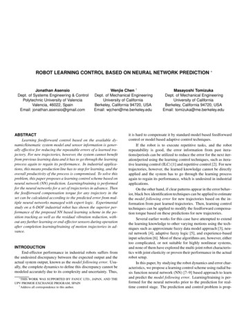
erly decoupled into sub-problems for each individual joint to reduce the algorithm complexity and computation requirements.The performance of the proposed approach is experimentallyevaluated and compared with the sensor based learning control,which requires learning for each new trajectory.qℓd,k 1P̂mu P̂ℓurq,k q̄md,k SYSTEM OVERVIEWConsider an n-joint robot with gear compliance. The robotis equipped with motor side encoders for real-time feedback, andan end-effector sensor (e.g., accelerometer) for off-line use. Notethat, if the computing resource and the sensor configuration allow, the end-effector sensor can also be used online. This paper, however, will address the conservative case where the endeffector sensor is for off-line and training use only, which is usually preferred in industry due to the cost saving and the limitedreal-time computational power.Robot Dynamic ModelThe dynamics of this robot can be formulated as [10]Mℓ (qℓ )q̈ℓ C(qℓ, q̇ℓ )q̇ℓ G(qℓ) Dℓ q̇ℓ Fℓc sgn(q̇ℓ )(1) T 1 1 J (qℓ ) fext KJ N qm qℓ DJ N q̇m q̇ℓ(2)Mm q̈m Dm q̇m Fmc sgn(q̇m ) τm 1 1 1 NKJ N qm qℓ DJ N q̇m q̇ℓwhere qℓ , qm Rn are the load side and the motor side position vectors, respectively. τm Rn is the motor torque vector.Mℓ (qℓ ) Rn n is the load side inertia matrix, C(qℓ , q̇ℓ ) Rn nis the Coriolis and centrifugal force matrix, and G(qℓ ) Rn isthe gravity vector. Mm , KJ , DJ , Dℓ , Dm , Fℓc , Fmc , and N Rn nare all diagonal matrices. The (i, i)-th elements of these matrices represent the motor side inertia, joint stiffness, joint damping, load side damping, motor side damping, load side Coulombfriction, motor side Coulomb friction, and gear ratio of the i-thjoint, respectively. fext R6 denotes the external force actingon the robot due to contact with the environment. The matrixJ(qℓ ) R6 n is the Jacobian matrix mapping from the load sidejoint space to the end-effector Cartesian space.Define the nominal load side inertia matrix as Mn diag(Mn1 , Mn2 , · · · , Mnn ) Rn n , where Mni Mℓ,ii (qℓ0 ), andMℓ,ii (qℓ0 ) is the (i, i)-th element of the inertia matrix Mℓ (qℓ0 )at the home (or nominal) position qℓ0 . Mn can be used to approximate the inertia matrix Mℓ (qℓ ). The off-diagonal entries ofMℓ (qℓ ) represent the coupling inertia between the joints. Then,the robot dynamic model can be reformulated as followsMm q̈m Dm q̇m τm Fmc sgn(q̇m ) N 1 KJ N 1 qm qℓ DJ N 1 q̇m q̇ℓMn q̈ℓ Dℓq̇ℓ d ℓ (q) KJ N 1 q m q ℓ DJ N 1q̇m q̇ℓ (3a)(3b)Figure 1. 1P̂mu qmd,k F1F2Cτln,k µkInner Plantdkτnl,kPmd Pℓd τm,k P Pmu ℓuqℓ,kqm,kτf b,k Robot control structure with reference & torque updateswhere all the coupling and nonlinear terms, such as Coriolis force, gravity, Coulomb frictions, and external forces, aregrouped into a fictitious disturbance torque d ℓ (q) Rn as d ℓ (q) Mn Mℓ 1 (qℓ ) In KJ N 1 qm qℓ DJ N 1 q̇m q̇ℓ Dℓ q̇ℓ Mn Mℓ 1 (qℓ ) C(qℓ , q̇ℓ )q̇ℓ G(qℓ) Fℓc sgn(q̇ℓ ) J T (qℓ ) fext(4) Twhere q qTm , qTℓ and In is an n n identity matrix.Thus, the robot can be considered as a MIMO system with2n inputs and 2n outputs as followsqm ( j) Pmu (z)τm ( j) Pmd (z)d( j)(5)qℓ ( j) Pℓu (z)τm ( j) Pℓd (z)d( j)(6)where j is the time index, z is the one step time advance operatorin the discrete time domain, and the fictitious disturbance inputd( j) is defined as Td( j) d(q( j)) [Fmc sgn(q̇m ( j))]T , [d ℓ (q( j))]T(7)The transfer functions from the inputs to the outputs (i.e.,Pmu , Pmd , Pℓu , and Pℓd ) can be derived from (3) as in [11].Controller Structure for Iterative Learning ControlNote that the robot dynamic model (3) is in a decoupled formsince all the variables are expressed in the diagonal matrix formor vector form. Therefore, the robot controller can be implemented in a decentralized form for each individual joint.Figure 1 illustrates the control structure for this robot system, where the subscript k is the iteration index. It consists oftwo feedforward controllers, F1 and F2 , and one feedback controller, C. Here, C can be any linear feedback controller suchas a decoupled PID controller to stabilize the system. The feedforward controllers, F1 and F2 , are designed using the nominalinverse model as 1qmd,k ( j) P̂mu (z)P̂ℓu(z)qℓd,k ( j) , F1 (z)qℓd,k ( j) 1τln,k ( j) P̂mu (z) qmd,k ( j) rq,k ( j) , F2 (z)q̄md,k ( j)(8)(9)

where ˆ is the nominal model representation of , and d isthe desired output of . rq,k and τnl,k are the additional reference and feedforward torque updates, respectively. The initialization/nominal values of these two updates are designed asFnlτnl,0Nonlinear ,0 N K̂J 1 (τ̂ℓdepℓ̈ M̂n q̈ℓd D̂ℓq̇ℓd )τnl,0 τ f f ,0 τ̂ln,0(10)P̂ℓ̈u q̈ ℓˆq̈ ℓ (11)/ŶǀĞƌƐĞ ŝŶĞŵĂƚŝĐƐp̈ewhereqℓdrq,0 q̄mdF2 1P̂muτ̂ℓd M̂ℓ (qℓd )q̈ℓd Ĉ(qℓd , q̇ℓd )q̇ℓd Ĝ(qℓd ) D̂ℓ q̇ℓd 1P̂mu P̂ℓu F̂ℓcsgn(q̇ℓd ) J T(qℓd ) fext,dτ̂md,0 M̂m q̈ md,0 D̂m q̇ md,0 F̂mc sgn(q̇ md,0 )(13)τ f f ,0 τ̂md,0 N 1 τ̂ℓd(14)(12) qmdC Inner Plantdτln ŶĚͲĞĨĨĞĐƚŽƌ ĐĐĞůĞƌŽŵĞƚĞƌτnl,1qℓµ τmPmd PℓdPmu Pℓuqmτf b F1Figure 2.Control diagram with neural network predictorIf the trajectory is repetitive, the two updates, rq,k and τnl,k ,can be generated iteratively by some ILC scheme such as thetwo-stage ILC algorithm designed in [11]. Particularly, the feedforward torque update τnl,k can be designed to compensate forthe model following error of the inner plant (shaded area in Fig.1) caused by the model uncertainty and the disturbance. This canbe realized using the plant inversion learning scheme [11], i.e.(11). The dashed lines indicate the parts when the end-effectorsensor is available and NN training can be conducted (e.g., inrobot factory tuning/testing stage). The training of the neural networks will be detailed later. The other parts with solid lines indicate the nominal control structure at the operation stage, wherethe NN predictor provides the model following error estimateê pℓ̈ for each joint for any trajectory in the set. The feedforwardtorque for a new trajectory is then computed as 1τnl,k 1 ( j) Qu (z)[τnl,k ( j) P̂ℓ̈u(z)e pℓ̈,k ( j)] 1(z)ê pℓ̈ ( j)]τnl,1 ( j) Qu (z)[τnℓ,0 ( j) P̂ℓ̈u(15)where Pℓ̈u is the transfer function from the motor torque τm to theload side joint acceleration q̈ℓ . The corresponding model following error is defined as e pℓ̈,k P̂ℓ̈u µk q̈ ℓ,k , where µk is the torqueinput to the inner plant and q̈ ℓ,k is the load side joint accelerationestimated from the end-effector accelerometer measurements using the inverse differential kinematics techniques such as the oneproposed in [12]. The low pass Q-filter Qu (z) is designed to tradeoff the performance bandwidth with the model uncertainties athigh frequencies. The stability assurance for the ILC schemeand the monotonic convergence of e pℓ̈,k are addressed in [11]. Itis shown that this torque update scheme is effective in reducingthe end-effector vibration, which is captured by the accelerometer.Controller Structure with Neural NetworksIf a new motion trajectory is desired, the prior ILC learning knowledge cannot be directly applied. Moreover, if the endeffector sensor is not available for executing the new task, themodel following error e pℓ̈,k cannot be obtained for new learningprocess. In this paper, we propose a neural network scheme topredict the model following error for a set of trajectories withoutfurther learning or end-effector sensor.Figure 2 shows the control diagram with neural network(NN) predictor for the feedforward torque update, where Fnl denotes the nominal nonlinear feedforward controller designed in(16)Note that if the end-effector sensor is available, the ILC process(15) with newly measured/calculated error information can stillcontinue after this initial run.NEURAL NETWORK PREDICTORIn this section a prediction system based on previously acquired training data is presented to estimate the joint acceleration model following error, which exhibits repeatable patternsunder certain conditions in the robot. Figure 3 shows the predictor structure with all the parts detailed below.Predictor Input DefinitionThe first step in this prediction problem is to choose the appropriate input signals that define the model following error. Inthis paper, we propose to define the predictor inputs as the trajectory references of either 2 dimensions (2D, velocity and acceleration) or 3 dimensions (3D, velocity, acceleration, and position).Moreover, due to the coupling dynamics on the multi-joint robot,a further study is carried out to identify the model following error as a proper combination of the trajectory references from alljoints together, which is termed as the movement cost in this paper.Proposition 1. The model following error e pℓ̈,0 when applying

Table 1.NN PredictorInput Definitionqℓd (j)MovementCostQiℓd (j)êipℓ̈ (j)Memoryif J A and J B are alignedJ A J BJ A J BDir iK(J A ) Dir iK(J B )1-1Dir iK(J A ) Dir iK(J B )-11Qiℓd (S)Pre-ProcessingDimension Normalization& Redefinition2D/3D(Sci )ExpertLogicNeural Network D/3D(SNN)NN4β0iif J A J B êipℓ̈ (S)Multiple NeuralNetwork Systemi12D/3D(SNN)Figure 3.PostProcessingNon-diagonal elements in matrix ΦExpandi1êipℓ̈ (SNN) êipℓ̈ (Sci )π20J A:Joint axis for which the movement cost is evaluatedJ B:Joint axis the effect of which over J A is assessedDir iK:Rotation direction when applying inverse kinematicsi2êipℓ̈ (SNN)i3êipℓ̈ (SNN)Ui4êipℓ̈ (SNN)Neural network predictor structurenominal feedforward torque τnl,0 is a function of the joint trajectory reference if the robot dynamics is repeatable.Proof. According to the control structure detailed in Fig. 1, themodel following error e pℓ̈,0 can be derived as(a) Axis Direction ConventionFigure 4.(b) Robot Home Position6-DOF robot example 1 1e pℓ̈,0 Pℓ̈u S p (C P̂mu)(P̂mu P̂ℓuqℓd rq,0 ) TuS p τnl,0 ( Pℓ̈u S pCPmd Pℓ̈d )d0(17)where S p (In CPmu ) 1 is the sensitivity function of the closedloop system, Tu P̂ℓ̈uCPmu Pℓ̈u , and Pℓ̈u Pℓ̈u P̂ℓ̈u ( [11]).From (8)-(14), rq,0 and τnl,0 are also the functions of qℓd .Moreover, if the robot dynamics is repeatable and the controllersetting remains the same, d0 will also be the function of qℓd .Thus, the model following error e pℓ̈,0 is a function of the jointreference qℓd . This proposition implies that during the identification ofe pℓ̈,0 based on qℓd , the feedback/feedforward controller and therobot working environment should remain consistent for all thetraining trajectories as well as the future desired task trajectories.Note that the robot dynamics is coupled among joints. Thus,due to rq,0 , τnl,0 , and d0 in (17), the model following error foreach joint depends on the reference trajectories of other joints aswell as that particular joint. In order to implement the decentralized predictor for each joint, the NN predictor input for the i-thjoint is designed as the movement cost position vector Qiℓd , velocity vector Q̇iℓd , and acceleration vector Q̈iℓd , which are definedas the linear combination of the reference trajectories across alljoints, i.e. Q1ℓd ( j)1 Q2 ( j) a21 ℓd . . . . Qnℓd ( j){z }Qℓd ( j) a121. 1 a1nqℓd ( j) 2 a2n qℓd ( j) . . . . an1 an2 . . . 1qn ( j){z} ℓd{z }Φ(18)qℓd ( j)Q̇ℓd ( j) Φ q̇ℓd ( j)(19)Q̈ℓd ( j) Φ q̈ℓd ( j)(20)where the design of Φ can be determined given a robot configuration. In this paper, we study the case of a 6-joint robotwhere the end-effector orientation is fixed as the home positionshown in Fig. 4. The diagonal elements of the matrix Φ areset to 1 since the movement cost on each joint depends directlyon its own movement. Non-diagonal elements are determinedas shown in Tab. 1 according to the convention of axis direction shown in Fig. 4 and the desired direction of joint rotation tomove the end-effector with fixed orientation.

Following this idea, the matrix Φ becomesTable 2. 1 0 01 01 0 1 1 0 1 0 0 1 1 0 1 0 Φ 1 0 0 1 0 1 0 1 1 0 1 0 1 0 01 01h i(21)Finally, the inputs to the prediction system are defined asthe velocity (19) and acceleration (20) movement costs for 2Dneural networks, or position (18), velocity (19), and acceleration(20) movement costs for 3D neural networks. The dimensionselection depends on the available training data and the computation power. It can be expected that a 3D network will generallyprovide more accurate prediction than a 2D network. However,more training data is required for a 3D network to perform effective learning. This also implies that more memory storage andcomputation capability are required for 3D networks.Data Pre-processingFor the neural network system to be effective, it is crucialthat there is a proper match between the data and neuron distribution in the input space. Hence, additional data pre-processingis developed to ensure that the training data covers all possibleinput values at which the neural network is intended to providea prediction. This pre-processing stage consists of a magnitudenormalization and variable redefinition of the input data, as wellas a filtering of the output data, i.e., the predicted model following error. It is aimed to simplify the complexity of the functionthat defines the model following error from the movement costs,and to standardize the neural network learning for optimal performance.Denote S as the set containing all the time steps, and T asthe total number of time steps for the executing trajectory. Thedata pre-processing stage is to setup the input signals υd,s for theNN predictor fNN , i.e.ê pℓ̈ ( j) Logic NotfNN (υ1,1 ( j), υ2,2 ( j), υ3,3 ( j)),3D NN (22a)fNN (υ2,2 ( j), υ3,3 ( j)),2D NN (22b)where j S {0, 1, 2, · · · , T }, the subscript d of υd,s denotesthe d-th dimension of the inputs, and s denotes the number ofpre-processing steps as explained below applied to this input dimension.Magnitude Normalization. First, for a given trajectorymovement costs (i.e., Qℓd , Q̇ℓd , and Q̈ℓd ), and the model following error e pℓ̈ to be learned by the neural network, a normalizationLogic and boolean operator symbols Logic AndLogic OrBoolean brackets with the output of as 0 or 1is applied to each input variable for the i-th joint, i.e. β0i max eipℓ̈(S) ,iυ2,1( j) Q̇iℓd ( j) ,max Q̇iℓd (S)iυ1,1( j) iυ3,1( j) Qiℓd ( j) ,max Qiℓd (S)Q̈iℓd ( j) max Q̈iℓd (S)(23)where max( ) denotes the maximum absolute value across thetime series .Prediction Viability Prediction is only viable while theend-effector is moving, since it is based on velocity and acceleration references. The viability condition, χci , is defined asχci ( j) iiυ2,1( j) ε2,1 jci Sci j : χci ( j) S iiυ3,1( j) ε3,1(24)(25)where the logic and boolean operators are defined as in Tab. 2.i and ε i are small positive numbers to check if a number isε2,13,1close to zero. Sci , as a subset of S, encloses the time steps jci thatare eligible to be processed for the prediction at the i-th joint.Redefinition on Acceleration Dimension In practice, reference trajectories are generated to ensure smooth motion. Thus acceleration and velocity pose a parabolic relationshipon the plane where the horizontal and the vertical axes are velocity and acceleration respectively (see Fig. 7(a) for example). Bystudying the experimental error characteristics, we note that themodel following error depends on the ratio between the velocity and the acceleration movement costs more significantly thanon any of these two inputs separately. To utilize this pattern, thethird dimension (acceleration movement cost) is redefined below.1. Change the third dimension to the arctangent betweenthe acceleration and the velocity movement costs, whichigives the result in the range of ( π2 , π2 ), i.e., υ3,2( jci ) !iiυ3,1 ( jc )arctan.i ( ji )υ2,1c2. Normalize the resulting third input dimension, i.e.,i ( j i ) 2 υ i ( j i ).υ3,3cπ 3,2 cNormalize Second Input Dimension To distributedata uniformly along all the input space, we need to normalize the second input dimension (velocity movement cost) at each

Table 3.i are introduced to describe theThen the boolean functions χ p, following specific circumstances in the input data using the logicand boolean operators defined in Tab. 2:Neural network activation ruleNN TypeVelocityAccelerationMotion eNegativeAcceleratingi χ p,AZ: Acceleration is constant & close to zero, i.e.,DE D hiEi ( ji ) i ( ji ) ε ii ( ji ) ε iχ p,AZυ3,3 υ3,3ccc3,3 ,3,3 ,sampled level of the third input dimension, i.e.i ( ji )υ2,1 c,l i (Si )max υ2,1c,l i jc : al υ3,3 ( jci ) bl Sciiiυ2,2( jc,l) ii jc,l Sc,l(26)(27)where l is the level number, al and bl are the bounds of the thirdinput dimension for the l-th level.This concludes the data pre-processing and the final predictor is formulated as in (22a)-(22b). Note that for the time stepswhere the joint remains static, no joint prediction is available,i ) 0, j i ii.e., êipℓ̈ ( jncnc / Sc .Multiple Neural Network ActivationIn order to enhance the prediction performance, the problemis divided into smaller prediction problems by means of multiple neural networks. Prior knowledge about the error behaviorbased on experience is formulated as several expert logic rules,whereby each network is specialized to a selected set of inputdata characterized by similar model following error behaviorsunder the movement cost definition. Here, each neural networkis confined to a different motion stage according to the signs ofthe velocity and the acceleration movement costs as described inTab. 3. In this way, the neural networks can learn all nonlinearities (e.g., Coulomb friction effect) more effectively in differentmotion stages.By exploring the robot dynamics and error characteristics,it is noted that the e pℓ̈ peaks normally appear when motionstarts/stops where strong acceleration is imposed, or when thejoint ends accelerating or starts decelerating where accelerationvaries exponentially. In addition, an exception is studied wherevelocity remains almost constant for long periods. In this region,e pℓ̈ tends to zero since the standard feedback and feedforwardcontroller is normally designed to achieve satisfactory steadystate performance.Define the pseudo-gradient and the pseudo-hessian for thethird dimension input signal as i ii υ3,3( jci ) υ3,3( jci ) υ3,3( jci 1) iiii 2 υ3,3( jci ) υ3,3( jci ) 2 υ3,3( jci 1) υ3,3( jci 2)(28)(29)i and ε iwhere ε3,3 ,3,3 are small numbers.i χ p,VC : Velocity remains constant for a long period, i.e.,acceleration is close to zero for a long period, which canibe obtained by analyzing χ p,AZvia Dilate and Erode imageprocessing methods [13].i χ p,AS: Acceleration changes sign, i.e., acceleration isclose to zeroDfor a short Eperiod,i ( ji ) χ ii ( ji )χ p,AS( jci ) χ p,AZccp,VCDEiii ( ji ) 0 . χ p,V p : Positive velocity, i.e., χ p,V p ( jci ) υ2,2cDEiiii χ p,V n : Negative velocity, i.e., χ p,V n ( jc ) υ2,2 ( jci ) 0 .i χ p,A: Initial acceleration, or concave accelerationi ( ji ) when velocity is close to be constant, i.e., χ p,AcDE D hiEii2iiiiυ3,3 ( jc ) 0 υ3,3 ( jc ) 0 χ p,AZ ( jc )i χ p,D: Final deceleration, or convex accelerationi ( ji ) when velocity is close to be constant, i.e., χ p,DcDE D hiEi ( j i ) 0 2 υ i ( j i ) 0 χ i ( j i )υ3,3cc3,3 cp,AZThen each of the four neural networks can be activated byitthe boolean function χNNdefined by the following rule, wherethe superscript t is the type of neural network defined in Tab. 3.i1 iii( jc ) χ p,AS ( jci ) χ p,A ( jci ) h χ p,VC ( jci )i χ p,VχNNp ( jc )i2 iii( jc ) χ p,AS ( jci ) χ p,D ( jci ) h χ p,VC ( jci )i χ p,VχNNp ( jc )i3 iiiχNN( jc ) χ p,AS ( jci ) χ p,D ( jci ) h χ p,VC ( jci )i χ p,Vn ( jc )i4 iiiχNN( jc ) χ p,AS ( jci ) χ p,A ( jci ) h χ p,VC ( jci )i χ p,Vn ( jc ) itititjNN SNN jci : χNN( jci ) SciThe model following error prediction from the t-th neuralit isnetwork on the i-th joint for the time steps enclosed by SNNitdenoted as ê pℓ̈ (SNN ). Note that when velocity is constant fora long period, ê pℓ̈ prediction is set to zero, i.e, êipℓ̈ ( jni NN ) 0, i1 S i2 S i3 S i4 jni NN / SNNSNN SNN SNN .Radial Basis Function Neural NetworkWith the identified error patterns, the radial basis functionneural networks [7, 8] can be applied to effectively learn themodel following error. The success of prediction relies on theNN learning method utilized to ensure a stable learning process [9].The neural networks utilized here are composedof two layers, and based on the radial basis function

(RBF) in (30).Define the t-th neural network for theitititi-th joint as fNN,RBF( x i ( jNN), θ it , µ it , σ it ), where x i ( jNN)iitiitTis either [υ2,2 ( jNN ), υ3,3 ( jNN )]for 2D networks, oriitiitiitT[υ1,1 ( jNN ), υ2,2 ( jNN ), υ3,3 ( jNN )] for 3D networks. DenoteD as the number of the input dimensions and md as the numberof neurons in the d-th dimension. Thus, the total number ofRBF neurons at the input layer is NRBF Dd 1 md . For the m-thneuron, the center position of the RBF and its width are presetand denoted respectively as µm RD and σm R. The neuralnetwork output, scaled by β0i R, is then defined in (31) asa product of the neuron regression vector, Γ it RNRBF 1 , andthe parameter vector, θ it RNRBF 1 , where the last entry θ0itcorresponds to the offset in the output prediction.fr ( x, µ , σ ) ek x µ k22 σ2(30) itititê pi ℓ̈ ( jNN) β0i θ it Γ it xi ( jNN), µ it , σ θ it θ it , · · · , θNit , θ it10RBF it ), fr ( x i ( jNNµ1it , σ1it ) . . Γ it ( x i ( j it ), µ it , σ it ) NN fr ( x i ( j it ), µ it , σ it ) NRBFNRBFNN1(31)(32)(33)The parameter vector θ it is tuned to minimize the followingquadratic cost function, VTit , using the training data with the actual model following error collected by the end-effector sensorand the inverse differential kinematics method proposed in [12],as the dashed part in Fig. 2.VTit 12 ititjNN SNN 2iiteNN( jNN)(34)i ( j it ) is the prediction error given the current where eNNθ it , i.e.,NNi ( j it ) e i ( j it ) ê i ( j it ). The optimized eNNθ it for this leastNNpℓ̈ NNpℓ̈ NNsquares problem can be numerically obtained by gradient methodwith momentum [14–16] using heuristically adaptive step sizeand momentum gain.Data Post-processingA zero-phase low-pass filter is applied to smooth the finaloutput of the NN predictor, which may contain discontinuitiesresulted from the output switching among neural networks andthe unavailability of prediction during the static periods. Thecut-off frequency for this low-pass filter is set to be higher thanthat of the Q-filter in (16) to ensure that the predicted informationis rich enough for control puGauge3DMeasurementSystemYZXOFigure 5.FANUC M-16iB robot systemDISCUSSION OF THE APPROACHStability & Safety AnalysisThe assurance of stability for this neural network basedlearning control as well as several safety measures are taken intoaccount during the design. On one hand, optimality and stabilityof the neural network training are ensured by utilizing radial basis function neurons in a double layer network with a quadraticcost function and momentum gradient method [15, 16]. On theother hand, the stability of plant inversion learning control (15)(16) is assured as detailed in [11].Furthermore, in order to increase prediction safety, data redundancy is utilized at the learning stage, and prediction uncertainty is also considered at the error prediction and feedforwardcorrection stage. Thus, as the uncertainty grows, the predictiontends to zero, and no feedforward torque modification is applied.Memory & Computation RequirementsThe presented approach is suited for centralized systemswhere online equipment such as the data acquisition target androbot controller have very limited computation and storage resources but a computer with higher resources is available for offline learning/training computation. In this way, one computercould be utilized for neural network training and learning control of several different robots for cost saving. If computationpower and storage resources are quite limited (i.e., off-line PC isnot available), some extra customization and simplification measures could be taken to facilitate the practical implementation.EXPERIMENTAL STUDYTest SetupThe proposed method is implemented on a 6-joint industrialrobot, FANUC M-16iB/20, in Fig. 5. The robot is equipped withbuilt-in motor encoders for each joint. An inertia sensor (AnalogDevices, ADIS16400) consisting of a 3-axial accelerometer anda 3-axial gyroscope is attached to the end-effector. The threedimensional position measurement system, CompuGauge 3D, isutilized to measure the end-effector tool center point (TCP) position as a ground truth for performance validation. The sampling

Table 4.Neuron distribution ranges for each neural networkNN Type1st Dimension2nd Dimension3rd Dimension1[ 1, 1][0, 1][ 0.1, 1]2[ 1, 1][0, 1][ 1, 0.1]3[ 1, 1][ 1,0][ 1, 0.1]4[ 1, 1][ 1,0][ 0.1, 1]Acc. (rad/s2)(a)(b)100 10 0.4 0.20Pos. (rad)Figure 6.0.2 0.50.50Vel. (rad/s)Training (blue) and validation (red) trajectories for Joint 3,based on a set of joint position, velocity, and acceleration referencesrates of all the sensor signals as well as the real-time controllerimplemented through MATLAB xPC Target are set to 1kHz.Algorithm SetupFor learning control algorithms (15)-(16), the zero-phaseacausal low-pass filter Qu is set with a cut-off frequency of 20Hz.The cut-off frequency for the NN output filtering is set to 50Hz.In order to train the neural networks

Polytechnic University of Valencia Valencia, 46022, Spain Email: jonathan.asensio@gmail.com Wenjie Chen Dept. of Mechanical Engineering University of California Berkeley, California 94720, USA Email: wjchen@me.berkeley.edu Masayoshi Tomizuka Dept. of Mechanical Engineering University of California Berkeley, California 94720, USA