Transcription
Chapter 7Laplace TransformThe Laplace transform can be used to solve differential equations. Besides being a different and efficient alternative to variation of parameters and undetermined coefficients, the Laplace method is particularlyadvantageous for input terms that are piecewise-defined, periodic or impulsive.The direct Laplace transform or the Laplace integral of a functionf (t) defined for 0 t is the ordinary calculus integration problemZ f (t)e st dt,0succinctly denoted L(f (t)) in science and engineering literature. TheL–notation recognizes that integration always proceeds over t 0 tot and that the integral involves an integrator e st dt instead of theusual dt. These minor differences distinguish Laplace integrals fromthe ordinary integrals found on the inside covers of calculus texts.7.1 Introduction to the Laplace MethodThe foundation of Laplace theory is Lerch’s cancellation lawR 0(1)y(t)e st dt R L(y(t) L(f (t))0f (t)e st dtimpliesorimpliesy(t) f (t),y(t) f (t).In differential equation applications, y(t) is the sought-after unknownwhile f (t) is an explicit expression taken from integral tables.Below, we illustrate Laplace’s method by solving the initial value problemy 0 1, y(0) 0.The method obtains a relation L(y(t)) L( t), whence Lerch’s cancellation law implies the solution is y(t) t.The Laplace method is advertised as a table lookup method, in whichthe solution y(t) to a differential equation is found by looking up theanswer in a special integral table.
7.1 Introduction to the Laplace Method247R g(t)e st dt is called the LaplaceRintegral of the function g(t). It is defined by limN 0N g(t)e st dt anddepends on variable s. The ideas will be illustrated for g(t) 1, g(t) tand g(t) t2 , producing the integral formulas in Table 1.Laplace Integral. The integralR 0R 0(1)e st dt (1/s)e st(t)e st dt R 0Assumed s 0.d(e st )dt dsd ds 0Laplace integral of g(t) 1. 1/s R t t 0(t2 )e st dtR 0 (1)e st dt0Used st )dt0 ds (ted R st dt ds0 (t)ed(1/s2 ) ds2/s31sdds F (t, s)dt ddsRF (t, s)dt.Differentiate.R (1)e st dt RUse L(1) 1/s.Table 1. The Laplace integralR Laplace integral of g(t) t.d(1/s) ds1/s2 0R 0R 0Laplace integral of g(t) t2 .Use L(t) 1/s2 .g(t)e st dt for g(t) 1, t and t2 .(t)e st dt 1s2In summary, L(tn ) R 0n!(t2 )e st dt 2s3s1 nAn Illustration. The ideas of the Laplace method will be illustrated for the solution y(t) t of the problem y 0 1, y(0) 0. Themethod, entirely different from variation of parameters or undeterminedcoefficients, uses basic calculus and college algebra; see Table 2.Table 2. Laplace method details for the illustration y 0 1, y(0) 0.y 0 (t)e st e stMultiply y 0 1 by e st .R Integrate t 0 to t .R0 st dt e st dt0 y (t)e0R 0 st dt 1/sy(t)e0Rs 0 y(t)e st dt y(0) 1/sR st dt 1/s20 y(t)eR R st dt ( t)e st dt0 y(t)e0y(t) tUse Table 1.Integrate by parts on the left.Use y(0) 0 and divide.Use Table 1.Apply Lerch’s cancellation law.
248Laplace TransformIn Lerch’s law, the formal rule of erasing the integral signs is valid provided the integrals are equal for large s and certain conditions hold on yand f – see Theorem 2. The illustration in Table 2 shows that Laplacetheory requires an in-depth study of a special integral table, a tablewhich is a true extension of the usual table found on the inside coversof calculus books. Some entries for the special integral table appear inTable 1 and also in section 7.2, Table 4.The L-notation for the direct Laplace transform produces briefer details,as witnessed by the translation of Table 2 into Table 3 below. The readeris advised to move from Laplace integral notation to the L–notation assoon as possible, in order to clarify the ideas of the transform method.Table 3. Laplace method L-notation details for y 0 1, y(0) 0translated from Table 2.L(y 0 (t)) L( 1)Apply L across y 0 1, or multiply y 0 1 by e st , integrate t 0 to t .L(y 0 (t)) 1/sUse Table 1.sL(y(t)) y(0) 1/sIntegrate by parts on the left.L(y(t)) 1/s2Use y(0) 0 and divide.L(y(t)) L( t)Apply Table 1.y(t) tInvoke Lerch’s cancellation law.Some Transform Rules. The formal properties of calculus integralsplus the integration by parts formula used in Tables 2 and 3 leads to theserules for the Laplace transform:L(f (t) g(t)) L(f (t)) L(g(t))The integral of a sum is thesum of the integrals.L(cf (t)) cL(f (t))Constants c pass through theintegral sign.L(y 0 (t)) sL(y(t)) y(0)The t-derivative rule, or integration by parts. See Theorem 3.Lerch’s cancellation law. SeeTheorem 2.L(y(t)) L(f (t)) implies y(t) f (t)1 Example (Laplace method) Solve by Laplace’s method the initial valueproblem y 0 5 2t, y(0) 1.Solution: Laplace’s method is outlined in Tables 2 and 3. The L-notation ofTable 3 will be used to find the solution y(t) 1 5t t2 .
7.1 Introduction to the Laplace MethodL(y 0 (t)) L(5 2t)25L(y 0 (t)) 2s s52sL(y(t)) y(0) 2s s152L(y(t)) 2 3s ssL(y(t)) L(1) 5L(t) L(t2 )2 L(1 5t t )y(t) 1 5t t2249Apply L across y 0 5 2t.Use Table 1.Apply the t-derivative rule, page 248.Use y(0) 1 and divide.Apply Table 1, backwards.Linearity, page 248.Invoke Lerch’s cancellation law.2 Example (Laplace method) Solve by Laplace’s method the initial valueproblem y 00 10, y(0) y 0 (0) 0.Solution: The L-notation of Table 3 will be used to find the solution y(t) 5t2 .L(y 00 (t)) L(10)Apply L across y 00 10.sL(y 0 (t)) y 0 (0) L(10)s[sL(y(t)) y(0)] y 0 (0) L(10)s2 L(y(t)) L(10)10L(y(t)) 3sL(y(t)) L(5t2 )Apply the t-derivative rule to y 0 , that is,replace y by y 0 on page 248.Repeat the t-derivative rule, on y.Use y(0) y 0 (0) 0.Use Table 1. Then divide.Apply Table 1, backwards.y(t) 5t2Invoke Lerch’s cancellation law.R e st f (t) dtis known to exist in the sense of the improper integral definition1Existence of the Transform. The Laplace integralZ g(t)dt limZNN 000g(t)dtprovided f (t) belongs to a class of functions known in the literature asfunctions of exponential order. For this class of functions the relation(2)f (t) 0t eatlimis required to hold for some real number a, or equivalently, for someconstants M and α,(3) f (t) M eαt .In addition, f (t) is required to be piecewise continuous on each finitesubinterval of 0 t , a term defined as follows.1An advanced calculus background is assumed for the Laplace transform existenceproof. Applications of Laplace theory require only a calculus background.
250Laplace TransformDefinition 1 (piecewise continuous)A function f (t) is piecewise continuous on a finite interval [a, b] provided there exists a partition a t0 · · · tn b of the interval [a, b]and functions f1 , f2 , . . . , fn continuous on ( , ) such that for t nota partition point(4) f1 (t).f (t) . fn (t)t0 t t1 ,.tn 1 t tn .The values of f at partition points are undecided by equation (4). Inparticular, equation (4) implies that f (t) has one-sided limits at eachpoint of a t b and appropriate one-sided limits at the endpoints.Therefore, f has at worst a jump discontinuity at each partition point.3 Example (Exponential order) Show that f (t) et cos t t is of exponential order, that is, show that f (t) is piecewise continuous and find α 0such that limt f (t)/eαt 0.Solution: Already, f (t) is continuous, hence piecewise continuous. FromL’Hospital’s rule in calculus, limt p(t)/eαt 0 for any polynomial p andany α 0. Choose α 2, thenlimt cos ttf (t) lim lim 2t 0.2ttt t eeeTheorem 1 (Existence of L(f ))Let f (t) be piecewise continuous on every finite interval in t 0 and satisfy f (t) M eαt for some constants M and α. Then L(f (t)) exists for s αand lims L(f (t)) 0.Proof: It has to be shown that the Laplace integral of f is finite for s α.Advanced calculus implies that it is sufficient to show that the integrand is absolutely bounded above by an integrable function g(t). Take g(t) M e (s α)t .Then g(t) 0. Furthermore, g is integrable, becauseZ Mg(t)dt .s α0Inequality f (t) M eαt implies the absolute value of the Laplace transformintegrand f (t)e st is estimated byf (t)e st M eαt e st g(t).M, because thes αright side of this inequality has limit zero at s . The proof is complete.The limit statement follows from L(f (t)) R 0g(t)dt
7.1 Introduction to the Laplace Method251Theorem 2 (Lerch)RIf f (t) and f2 (t) are continuous, of exponential order and 0 f1 (t)e st dt R 1 st dt for all s s , then f (t) f (t) for t 0.0120 f2 (t)eProof: See Widder [?].Theorem 3 (t-Derivative Rule)If f (t) is continuous, lim f (t)e st 0 for all large values of s and f 0 (t)t is piecewise continuous, then L(f 0 (t)) exists for all large s and L(f 0 (t)) sL(f (t)) f (0).Proof: See page 276.Exercises 7.1PNSolve the given 18. f (t) n 1 cn sin(nt), for anychoice of the constants c1 , . . . , cN .initial value problem using Laplace’smethod.Existence of transforms. Let f (t) 1. y 0 2, y(0) 0.22tet sin(et ). Establish these results.2. y 0 1, y(0) 0.19. The function f (t) is not of expo-Laplace method.nential order.3. y 0 t, y(0) 0.20. Theintegral of f (t),R Laplace stf(t)edt,converges for all0s 0.4. y 0 t, y(0) 0.5. y 0 1 t, y(0) 0.6. y 0 1 t, y(0) 0.7. y 0 3 2t, y(0) 0.8. y 0 3 2t, y(0) 0.0009. y 2, y(0) y (0) 0.00010. y 1, y(0) y (0) 0.00011. y 1 t, y(0) y (0) 0.12. y 00 1 t, y(0) y 0 (0) 0.00000013. y 3 2t, y(0) y (0) 0.14. y 3 2t, y(0) y (0) 0.Jump Magnitude. For f piecewisecontinuous, define the jump at t byJ(t) lim f (t h) lim f (t h).h 0 h 0 Compute J(t) for the following f .21. f (t) 1 for t 0, else f (t) 022. f (t) 1 for t 1/2, else f (t) 023. f (t) t/ t for t 6 0, f (0) 024. f (t) sin t/ sin t for t 6 nπ,f (nπ) ( 1)n.P seriesExponential order. Show that f (t) TaylornThe series relationP nL( n 0 cn t ) n 0 cn L(t ) oftenis of exponential order, by finding aholds, in which case the result L(tn ) constant α 0 in each case such thatn!s 1 n can be employed to find af (t) 0.limseries representation of the Laplacet eαttransform. Use this idea on the fol15. f (t) 1 tlowing to find a series formula forL(f (t)).16. f (t) et sin(t)P 2tnPN17. f (t) n 0 cn xn , for any choice 25. f (t) e n 0 (2t) /n!P of the constants c0 , . . . , cN .26. f (t) e t n 0 ( t)n /n!
252Laplace Transform7.2 Laplace Integral TableThe objective in developing a table of Laplace integrals, e.g., Tables 4and 5, is to keep the table size small. Table manipulation rules appearing in Table 6, page 257, effectively increase the table size manyfold,making it possible to solve typical differential equations from electricaland mechanical problems. The combination of Laplace tables plus thetable manipulation rules is called the Laplace transform calculus.Table 4 is considered to be a table of minimum size to be memorized.Table 5 adds a number of special-use entries. For instance, the Heavisideentry in Table 5 is memorized, but usually not the others.Derivations are postponed to page 270. The theory of the gamma function Γ(x) appears below on page 255.Table 4. A minimal Laplace integral table with L-notationR 0R 0(tn )e st dt (eat )e st dt n!1s a0(cos bt)e st dt s1 nL(eat ) s b2R b stdt 20 (sin bt)es b2R n!L(tn ) s1 n1s as b2bL(sin bt) 2s b2L(cos bt) s2s2Table 5. Laplace integral table extensionL(H(t a)) e as(a 0)sL(δ(t a)) e asL(floor(t/a)) e ass(1 e as )L(sqw(t/a)) 1tanh(as/2)sL(a trw(t/a)) 1tanh(as/2)s2Γ(1 α)s1 αrπ 1/2L(t) sL(tα ) Heaviside unit step, defined by1for t 0,H(t) 0otherwise.Dirac delta, δ(t) dH(t).Special usage rules apply.Staircase function,floor(x) greatest integer x.Square wave,sqw(x) ( 1)floor(x) .TriangularRwave,xtrw(x) 0 sqw(r)dr.Generalized powerR function,Γ(1 α) 0 e x xα dx.Because Γ(1/2) π.
7.2 Laplace Integral Table2534 Example (Laplace transform) Let f (t) t(t 1) sin 2t e3t . ComputeL(f (t)) using the basic Laplace table and transform linearity properties.Solution:L(f (t)) L(t2 5t sin 2t e3t )2Expand t(t 5).3t L(t ) 5L(t) L(sin 2t) L(e )2521 3 2 2 sss 4 s 3Linearity applied.Table lookup.5 Example (Inverse Laplace transform) Use the basic Laplace table backwards plus transform linearity properties to solve for f (t) in the equationL(f (t)) s2s2s 1 3 . 16 s 3sSolution:111 2s 2 2 16s 3 s2 s33t L(cos 4t) 2L(e ) L(t) 12 L(t2 )L(f (t)) s23t L(cos 4t 2e t 3tf (t) cos 4t 2e t 1 22t )1 22tConvert to table entries.Laplace table (backwards).Linearity applied.Lerch’s cancellation law.6 Example (Heaviside) Find the Laplace transform of f (t) in Figure 1.51135Figure 1. A piecewise definedfunction f (t) on 0 t : f (t) 0except for 1 t 2 and 3 t 4.Solution: The details require the use of the Heaviside function formulaH(t a) H(t b) The formula for f (t): 1 1 t 2,153 t 4,f (t) 0 0 otherwise 1 a t b,0 otherwise.1 t 2, 5otherwise 103 t 4,otherwiseThen f (t) f1 (t) 5f2 (t) where f1 (t) H(t 1) H(t 2) and f2 (t) H(t 3) H(t 4). The extended table givesL(f (t)) L(f1 (t)) 5L(f2 (t)) L(H(t 1)) L(H(t 2)) 5L(f2 (t))Linearity.Substitute for f1 .
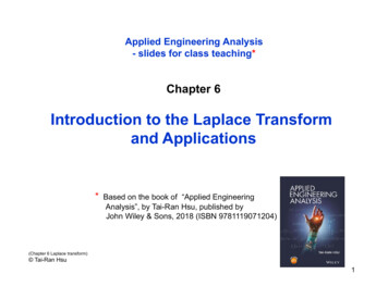
254Laplace Transforme s e 2s 5L(f2 (t))se s e 2s 5e 3s 5e 4s s Extended table used.Similarly for f2 .7 Example (Dirac delta) A machine shop tool that repeatedly hammers aPdie is modeled by the Dirac impulse model f (t) Nn 1 δ(t n). ShowPN nsthat L(f (t)) n 1 e .Solution: P NL(f (t)) Lδ(t n)n 1PN n 1 L(δ(t n))P ns Nn 1 eLinearity.Extended Laplace table.8 Example (Square wave) A periodic camshaft force f (t) applied to a mechanical system has the idealized graph shown in Figure 2. Show thatf (t) 1 sqw(t) and L(f (t)) 1s (1 tanh(s/2)).201Figure 2. A periodic force f (t) appliedto a mechanical system.3Solution:1 sqw(t) 1 11 12n t 2n 1, n 0, 1, . . .,2n 1 t 2n 2, n 0, 1, . . ., 20 f (t). 2n t 2n 1, n 0, 1, . . .,otherwise,By the extended Laplace table, L(f (t)) L(1) L(sqw(t)) 1 tanh(s/2) .ss9 Example (Sawtooth wave) Express the P -periodic sawtooth wave represented in Figure 3 as f (t) ct/P c floor(t/P ) and obtain the formulaL(f (t)) ce P sc .P s2 s se P sc0P4PFigure 3. A P -periodic sawtoothwave f (t) of height c 0.
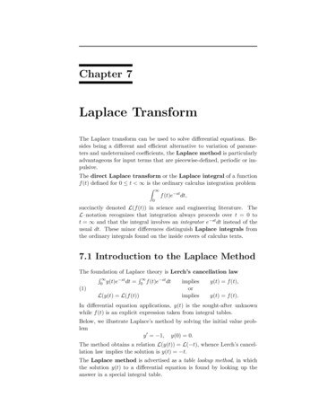
7.2 Laplace Integral Table255Solution: The representation originates from geometry, because the periodicfunction f can be viewed as derived from ct/P by subtracting the correct constant from each of intervals [P, 2P ], [2P, 3P ], etc.The technique used to verify the identity is to define g(t) ct/P c floor(t/P )and then show that g is P -periodic and f (t) g(t) on 0 t P . Two P periodic functions equal on the base interval 0 t P have to be identical,hence the representation follows.The fine details: for 0 t P , floor(t/P ) 0 and floor(t/P k) k. Henceg(t kP ) ct/P ck c floor(k) ct/P g(t), which implies that g isP -periodic and g(t) f (t) for 0 t P .cL(t) cL(floor(t/P ))Pcce P s P s2s se P sL(f (t)) Linearity.Basic and extended table applied.10 Example (Triangular wave) Express the triangular wave f of Figure 4 in5terms of the square wave sqw and obtain L(f (t)) 2 tanh(πs/2).πs50Figure 4. A 2π-periodic triangularwave f (t) of height 5.2πSolution: The representation of f in terms of sqw is f (t) 5R t/π0sqw(x)dx.Details: A 2-periodic triangular wave of height 1 is obtained by integratingthe square wave of period 2. A wave of height c and period 2 is given byRtR 2t/Pc trw(t) c 0 sqw(x)dx. Then f (t) c trw(2t/P ) c 0sqw(x)dx wherec 5 and P 2π.Laplace transform details: Use the extended Laplace table as follows.L(f (t)) 55L(π trw(t/π)) 2 tanh(πs/2).ππsGamma Function. In mathematical physics, the Gamma function or the generalized factorial function is given by the identity(1)Γ(x) Z e t tx 1 dt,x 0.0This function is tabulated and available in computer languages like Fortran, C and C . It is also available in computer algebra systems andnumerical laboratories. Some useful properties of Γ(x):(2)Γ(1 x) xΓ(x)(3)Γ(1 n) n! for integersn 1.
256Laplace TransformR e t dt 1, which givesΓ(1) 1. Use this identity and successively relation (2) to obtain relation (3).To prove identity (2), integration by parts is applied, as follows:R Γ(1 x) 0 e t tx dtDefinition.Rt tx e t t 0 0 e t xtx 1 dtUse u tx , dv e t dt.R t x 1 x 0 e tdtBoundary terms are zerofor x 0. xΓ(x).Details for relations (2) and (3): Start with0Exercises 7.2Laplacetransform.Compute Inverse Laplace transform. SolveL(f (t)) using the basic Laplace table the given equation for the functionand the linearity properties of the f (t). Use the basic table and linearitytransform. Do not use the direct properties of the Laplace transform.Laplace transform!21. L(f (t)) s 21. L(2t)22. L(f (t)) 4s 22. L(4t)23. L(f (t)) 1/s 2/s2 3/s323. L(1 2t t )24. L(f (t)) 1/s3 1/s24. L(t 3t 10)25. L(f (t)) 2/(s2 4)5. L(sin 2t)26. L(f (t)) s/(s2 4)6. L(cos 2t)27. L(f (t)) 1/(s 3)7. L(e2t )28. L(f (t)) 1/(s 3)8. L(e 2t )29. L(f (t)) 1/s s/(s2 4)9. L(t sin 2t)30. L(f (t)) 2/s 2/(s2 4)10. L(t cos 2t)31. L(f (t)) 1/s 1/(s 3)11. L(t e2t )32. L(f (t)) 1/s 3/(s 2)12. L(t 3e 2t )33. L(f (t)) (2 s)2 /s313. L((t 1)2 )34. L(f (t)) (s 1)/s214. L((t 2)2 )35. L(f (t)) s(1/s2 2/s3 )15. L(t(t 1))36. L(f (t)) (s 1)(s 1)/s316. L((t 1)(t 2))P1037. L(f (t)) n 0 n!/s1 nP10 n17. L( n 0 t /n!)P1038. L(f (t)) n 0 n!/s2 nP10 n 118. L( n 0 t/n!)P10n39. L(f (t)) n 1 2P10s n219. L( n 1 sin nt)P10sP1040. L(f (t)) n 0 220. L( n 0 cos nt)s n2
7.3 Laplace Transform Rules2577.3 Laplace Transform RulesIn Table 6, the basic table manipulation rules are summarized. Fullstatements and proofs of the rules appear in section 7.7, page 275.The rules are applied here to several key examples. Partial fractionexpansions do not appear here, but in section 7.4, in connection withHeaviside’s coverup method.Table 6. Laplace transform rulesL(f (t) g(t)) L(f (t)) L(g(t))Linearity.L(cf (t)) cL(f (t))Linearity.L(y 0 (t)) sL(y(t)) y(0)The t-derivative rule. 1Lg(x)dx L(g(t))sdL(tf (t)) L(f (t))ds Rt0The Laplace of a sum is the sum of the Laplaces.Constants move through the L-symbol.Derivatives L(y 0 ) are replaced in transformed equations.The t-integral rule.The s-differentiation rule.Multiplying f by t applies d/ds to the transform of f .L(eat f (t)) L(f (t)) s (s a)First shifting rule.L(f (t a)H(t a)) e as L(f (t)),L(g(t)H(t a)) e as L(g(t a))RPf (t)e st dtL(f (t)) 01 e P sSecond shifting rule.L(f (t))L(g(t)) L((f g)(t))Convolution rule.RtMultiplying f by eat replaces s by s a.First and second forms.Rule for P -periodic functions.Assumed here is f (t P ) f (t).Define (f g)(t) 0f (x)g(t x)dx.11 Example (Harmonic oscillator) Solve by Laplace’s method the initial valueproblem x00 x 0, x(0) 0, x0 (0) 1.Solution: The solution is x(t) sin t. The details:L(x00 ) L(x) L(0)00sL(x ) x (0) L(x) 00s[sL(x) x(0)] x (0) L(x) 02(s 1)L(x) 11L(x) 2s 1 L(sin t)x(t) sin tApply L across the equation.Use the t-derivative rule.Use again the t-derivative rule.Use x(0) 0, x0 (0) 1.Divide.Basic Laplace table.Invoke Lerch’s cancellation law.
258Laplace Transform2.(s 5)312 Example (s-differentiation rule) Show the steps for L(t2 e5t ) Solution: dL(t e ) L(e5t )ds 12 d d ( 1)ds ds s 5 d 1 ds (s 5)22 (s 5)32 5td dsApply s-differentiation.Basic Laplace table.Calculus power rule.Identity verified.13 Example (First shifting rule) Show the steps for L(t2 e 3t ) 2.(s 3)3Solution:L(t2 e 3t ) L(t2 ) s s ( 3) 2 s2 1 s s ( 3) First shifting rule.Basic Laplace table.2(s 3)3Identity verified.14 Example (Second shifting rule) Show the steps forL(sin t H(t π)) e πs.s2 1Solution: The second shifting rule is applied as follows.L(sin t H(t π)) L(g(t)H(t a) e as L(g(t a) e πs e πs e πsChoose g(t) sin t, a π.Second form, second shifting theorem.L(sin(t π)) Substitute a π.L( sin t) 1s2 1Sum rule sin(a b) sin a cos b sin b cos a plus sin π 0, cos π 1.Basic Laplace table. Identity verified.15 Example (Trigonometric formulas) Show the steps used to obtain theseLaplace identities:32s 2 a22 cos at) 2(s 3sa )(a) L(t cos at) 2(c)L(t(s a2 )2(s2 a2 )3232sa2 sin at) 6s a a(d)L(t(b) L(t sin at) 2(s a2 )2(s2 a2 )3
7.3 Laplace Transform Rules259Solution: The details for (a):L(t cos at) (d/ds)L(cos at) sd ds s2 a2 s2 a 2(s2 a2 )2Use s-differentiation.Basic Laplace table.Calculus quotient rule.The details for (c):L(t2 cos at) (d/ds)L(( t) cos at) s2 a 2d 2 ds(s a2 )2 2s3 6sa2 )(s2 a2 )3Use s-differentiation.Result of (a).Calculus quotient rule.The similar details for (b) and (d) are left as exercises.16 Example (Exponentials) Show the steps used to obtain these Laplaceidentities:22s aat cos bt) (s a) b(c)L(te(a) L(eat cos bt) (s a)2 b2((s a)2 b2 )22b(s a)b(d) L(teat sin bt) (b) L(eat sin bt) (s a)2 b2((s a)2 b2 )2Solution: Details for (a):L(eat cos bt) L(cos bt) s s a s s2 b2 s s as a (s a)2 b2First shifting rule.Basic Laplace table.Verified (a).Details for (c):L(teat cos bt) L(t cos bt) s s a d L(cos bt)dss s a sd ds s2 b2s s a 2 s b2 (s2 b2 )2 s s a (s a)2 b2((s a)2 b2 )2Left as exercises are (b) and (d).First shifting rule.Apply s-differentiation.Basic Laplace table.Calculus quotient rule.Verified (c).
260Laplace Transform17 Example (Hyperbolic functions) Establish these Laplace transform factsabout cosh u (eu e u )/2 and sinh u (eu e u )/2.s 2 a2(s2 a2 )22as(d) L(t sinh at) 2(s a2 )2s2s a2a(b) L(sinh at) 2s a2(c) L(t cosh at) (a) L(cosh at) Solution: The details for (a):L(cosh at) 12 (L(eat ) L(e at )) 111 2 s a s as 2s a2Definition plus linearity of L.Basic Laplace table.Identity (a) verified.The details for (d): daL(t sinh at) ds s2 a2a(2s) 2(s a2 )2Apply the s-differentiation rule.Calculus power rule; (d) verified.Left as exercises are (b) and (c).18 Example (s-differentiation) Solve L(f (t)) (s22sfor f (t). 1)2Solution: The solution is f (t) t sin t. The details:2s(s2 1)2 d1 ds s2 1d (L(sin t))ds L(t sin t)L(f (t)) f (t) t sin tCalculus power rule (un )0 nun 1 u0 .Basic Laplace table.Apply the s-differentiation rule.Lerch’s cancellation law.19 Example (First shift rule) Solve L(f (t)) s 2for f (t).22 2s 2Solution: The answer is f (t) e t cos t e t sin t. The details:L(f (t)) s 2s2 2s 2s 2(s 1)2 1Signal for this method: the denominator has complex roots.Complete the square, denominator.
7.3 Laplace Transform Rules261S 1S2 11S 2S 1 S2 1 L(cos t) L(sin t) s S s 1 L(ef (t) e t tcos t) L(ecos t e t tsin t)sin tSubstitute S for s 1.Split into Laplace table entries.Basic Laplace table.First shift rule.Invoke Lerch’s cancellation law.20 Example (Damped oscillator) Solve by Laplace’s method the initial valueproblem x00 2x0 2x 0, x(0) 1, x0 (0) 1.Solution: The solution is x(t) e t cos t. The details:L(x00 ) 2L(x0 ) 2L(x) L(0)Apply L across the equation.s[sL(x) x(0)] x0 (0) 2[L(x) x(0)] 2L(x) 0The t-derivative rule on x.000The t-derivative rule on x0 .sL(x ) x (0) 2L(x ) 2L(x) 0(s2 2s 2)L(x) 1 ss 1L(x) 2s 2s 2s 1 (s 1)2 1Use x(0) 1, x0 (0) 1.Divide.Complete the square in the denominator.Basic Laplace table. L(cos t) s s 1 L(e t cos t)First shifting rule.x(t) e t cos tInvoke Lerch’s cancellation law.21 Example (Rectified sine wave) Compute the Laplace transform of therectified sine wave f (t) sin ωt and show it can be expressed in theformπs ω coth 2ω.L( sin ωt ) s2 ω 2Solution: The periodic function formula will be appliedwith period P RP2π/ω. The calculation reduces to the evaluation of J 0 f (t)e st dt. Becausesin ωt 0 on π/ω t 2π/ω, integral J can be written as J J1 J2 , whereJ1 Zπ/ωsin ωt e st dt,J2 0Z2π/ωπ/ω sin ωt e st dt.Integral tables give the resultZωe st cos(ωt) se st sin(ωt)sin ωt e st dt .s2 ω 2s2 ω 2ThenJ1 ω(e π s/ω 1),s2 ω 2J2 ω(e 2πs/ω e πs/ω ),s2 ω 2
262Laplace TransformJ ω(e πs/ω 1)2.s2 ω 2The remaining challenge is to write the answer for L(f (t)) in terms of coth.The details:L(f (t)) J1 e P s(1 Periodic function formula.Je P s/2 )(1Apply 1 x2 (1 x)(1 x),x e P s/2 . e P s/2 )ω(1 e P s/2 )(1 e P s/2 )(s2 ω 2 )Cancel factor 1 e P s/2 .eP s/4 e P s/4ωeP s/4 e P s/4 s2 ω 22 cosh(P s/4)ω 22 sinh(P s/4) s ω 2ω coth(P s/4) s2 ω 2 πsω coth 2ω s2 ω 2Factor out e P s/4 , then cancel. Apply cosh, sinh identities.Use coth u cosh u/ sinh u.Identity verified.22 Example (Half–wave rectification) Compute the Laplace transform of thehalf–wave rectification of sin ωt, denoted g(t), in which the negative cyclesof sin ωt have been canceled to create g(t). Show in particular that1 ωπsL(g(t)) 1 coth222s ω2ω Solution: The half–wave rectification of sin ωt is g(t) (sin ωt sin ωt )/2.Therefore, the basic Laplace table plus the result of Example 21 giveL(2g(t)) L(sin ωt) L( sin ωt )ωω cosh(πs/(2ω)) 2 2s ωs2 ω 2ω(1 cosh(πs/(2ω)) 2s ω2Dividing by 2 produces the identity.23 Example (Shifting rules) Solve L(f (t)) e 3ss2s 1for f (t). 2s 2Solution: The answer is f (t) e3 t cos(t 3)H(t 3). The details:s 1(s 1)2 1S e 3s 2S 1 e 3S 3 (L(cos t)) s S s 1L(f (t)) e 3sComplete the square.Replace s 1 by S.Basic Laplace table.
7.3 Laplace Transform Rules e3 e 3s L(cos t) s S s 1 e3 (L(cos(t 3)H(t 3))) s S s 13 e L(ef (t) e3 t tcos(t 3)H(t 3))cos(t 3)H(t 3)24 Example () Solve L(f (t) s2263Regroup factor e 3S .Second shifting rule.First shifting rule.Lerch’s cancellation law.s 7for f (t). 4s 8Solution: The answer is f (t) e 2t (cos 2t 52 sin 2t). The details:s 7(s 2)2 4S 5 2S 45 2S 2S 4 2 S2 4s5 2 2 s 4 2 s2 4 s S s 2L(f (t)) L(cos 2t) 25 L(sin 2t) L(ef (t) e 2t 2t(cos 2t (cos 2t 5252s S s 2sin 2t))sin 2t)Complete the square.Replace s 2 by S.Split into table entries.Prepare for shifting rule.Basic Laplace table.First shifting rule.Lerch’s cancellation law.
264Laplace Transform7.4 Heaviside’s MethodThis practical method was popularized by the English electrical engineerOliver Heaviside (1850–1925). A typical application of the method is tosolve2s L(f (t))(s 1)(s2 1)for the t-expression f (t) e t cos t sin t. The details in Heaviside’smethod involve a sequence of easy-to-learn college algebra steps.More precisely, Heaviside’s method systematically converts a polynomial quotienta0 a1 s · · · an sn(1)b0 b1 s · · · bm sminto the form L(f (t)) for some expression f (t). It is assumed thata0 , ., an , b0 , . . . , bm are constants and the polynomial quotient (1) haslimit zero at s .Partial Fraction TheoryIn college algebra, it is shown that a rational function (1) can be expressed as the sum of terms of the form(2)A(s s0 )kwhere A is a real or complex constant and (s s0 )k divides the denominator in (1). In particular, s0 is a root of the denominator in (1).Assume fraction (1) has real coefficients. If s0 in (2) is real, then A isreal. If s0 α iβ in (2) is complex, then (s s0 )k also appears, wheres0 α iβ is the complex conjugate of s0 . The corresponding termsin (2) turn out to be complex conjugates of one another, which can becombined in terms of real numbers B and C as(3)B CsAA .kk(s s0 )(s s0 )((s α)2 β 2 )kSimple Roots. Assume that (1) has real coefficients and the denominator of the fraction (1) has distinct real roots s1 , . . . , sN and distinctcomplex roots α1 iβ1 , . . . , αM iβM . The partial fraction expansionof (1) is a sum given in terms of real constants Ap , Bq , Cq by(4)NMXXApBq Cq (s αq )a0 a1 s · · · an sn .mb0 b1 s · · · bm ss sp q 1 (s αq )2 βq2p 1
7.4 Heaviside’s Method265Multiple Roots. Assume (1) has real coefficients and the denominator of the fraction (1) has possibly multiple roots. Let Np be themultiplicity of real root sp and let Mq be the multiplicity of complex rootαq iβq , 1 p N , 1 q M . The partial fraction expansion of (1)is given in terms of real constants Ap,k , Bq,k , Cq,k by(5)NXXp 1 1 k NpMXX Bq,k Cq,k (s αq )Ap,k .k(s sp )((s αq )2 βq2 )kq 1 1 k MqHeaviside’s Coverup MethodThe method applies only to the case of distinct roots of the denominatorin (1). Extensions to multiple-root cases can be made; see page 266.To illustrate Oliver Heaviside’s ideas, consider the problem details(6)2s 1s(s 1)(s 1)ABC ss 1 s 1 L(A) L(Bet ) L(Ce t ) L(A Bet Ce t )The first line (6) uses college algebra partial fractions. The second andthird lines use the Laplace integral table and properties of L.Heaviside’s mysterious method. Oliver Heaviside proposed tofind in (6) the constant C 12by a cover–up method:2s 1s(s 1) C.s 1 0The instructions are to cover–up the matching factors (s 1) on the left, then evaluate on the left at the root s whichand right with boxmakes the contents of the box zero. The other terms on the right arereplaced by zero.To justify Heaviside’s cover–up method, multiply (6) by the denominators 1 of partial fraction C/(s 1):(2s 1) (s 1)s(s 1) (s 1) A (s 1)s B (s 1)s 1 C (s 1)(s 1).Set (s 1) 0 in the display. Cancellations left and right plus annihilation of two terms on the right gives Heaviside’s prescription2s 1s(s 1) C.s 1 0 pag
3 Example (Exponential order) Show that f(t) et cost t is of expo-nential order, that is, show that f(t) is piecewise continuous and nd 0 such that limt!1 f(t) e t 0. Solution: Already, f(t) is continuous, hence piecewise continuous. From L'Hospital's rule in calculus, limt!1 p(t) e t 0 for any polynomial p and any 0. Choose 2 .