Transcription
Applied Engineering Analysis- slides for class teaching*Chapter 6Introduction to the Laplace Transformand Applications* Based on the book of “Applied EngineeringAnalysis”, by Tai-Ran Hsu, published byJohn Wiley & Sons, 2018 (ISBN 9781119071204)(Chapter 6 Laplace transform) Tai-Ran Hsu1
Chapter Learning Objectives Learn the application of Laplace transform in engineering analysis. Learn the required conditions for transforming variable or variables infunctions by the Laplace transform. Learn the use of available Laplace transform tables for transformationof functions and the inverse transformation. Learn to use partial fractions and convolution methods in inverse Laplacetransforms. Learn the Laplace transform for ordinary derivatives and partial derivatives ofdifferent orders. Learn how to use Laplace transform methods to solve ordinary and partialdifferential equations. Learn the use of special functions in solving indeterminate beam bendingproblems using Laplace transform methods.2
6.1IntroductionLaplace, Pierre-Simon (1749-1829)- a French mathematician, astronomerand statistician.Major accomplishments in mathematics: Laplace equation for electrical andmechanical potentials 2 P x, y 2 P x, y 0 x 2 y 2where P(x,y) Temperature for thermal potential or electric charge in electrostatics Laplacian differential operator: 2 2 22 2 2 2 x y z Laplace transform:orLx F x Lt f t 0 0, ande sx F x dxe st f t dt3where F(x) is a function of variable x and f(t) is a function of variable t, and s Laplace transform parameter
Laplace Transform in Engineering Analysis Laplace transform is a mathematical operation that is used to “transform” a variable(such as x, or y, or z in space, or at time t) to a parameter (s) – a “constant” under certainconditions. It transforms ONE variable at a time.Mathematically, it can be expressed as: (6.1)Lt f t e st f t dt F s 0 where F(s) expression of Laplace transform of function f(t) involving the parameter s In a layman’s term, Laplace transform is used to “transform” a variable in a functioninto a parameter - a parameter is a “constant” under certain conditions So, after the Laplace transformation that variable is no longer a variable anymore,but it should be treated as a “parameter”, i.e a “constant under specific conditions” This “specific condition” for the Laplace transform is: Laplace transform can only be used to transform variables that cover a range from“zero (0)” to infinity, ( ), for instance: 0 t if t is the variable to be transformed Any variable that does not vary within this range cannot be transformed usingLaplace transform Because time variable t is the most common variable that varies from (0 to ), functions withvariable t are commonly transformed by Laplace transform Lapalce transform is a valuable “tool” in solving: Differential equations for example: electronic circuit equations, and In “feedback control” for example, in stability and control of aircraft systems4
6.2Mathematical Operator of Laplace TransformThe Laplace transform of a function f(t) is designated as L[f(t)], with the variable t covers aspectrum of (0, ).The mathematical expression of the Laplace transform of this function with 0 t hasthe form:L f (t ) 0f (t ) e st dt F (s)(6.1)where s is the parameter of the Laplace transform, and F(s) is the expression of theLaplace transform of function f(t) with 0 t .The “inverse Laplace transform” operates in a reverse way; That is to invert thetransformed expression of F(s) in Equation (6.1) to its original function f(t). Mathematically,it has the form:L-1[F(s)] f(t)(6.2)The above definition of Laplace transform as expressed in Equation (6.1) provides us withthe “specific condition” for treating the Laplace transform parameter s as a constant is thatthe variable in the function to be transformed must SATISFY the condition that0 (variable t) 5
Examples 6.1 (p.172)Express the Laplace transforms of the following simple functions:(1) For f(t) t2L f (t ) with 0 t : e0 st t dt e2 st 2t 2 2t 2 2 3 s 2s s 0 2 F (s)3s(a)(2) For f(t) eat with a constant and 0 t :L f t 0 e st e at dt e s a t dt 011e s a s as a0(b)(3) For f(t) Cosωt with ω constant and 0 t :L Cos t e st Cos t dt 0 st es sCostSint 22s s 2 20(c)Appendix 1 of the book provides a Table of Laplace transforms of simple functions (p.463)For example, L[f(t)] of a polynomial t2 in Equation (a) is Case 3 with n 3 in the Table,exponential function eat in Equation (b) is Case 7, andtrigonometric function Cosωt in Equation (c) is Case 186
Example 6.2 (p.172)Perform the Laplace transform on the ramp function illustrated below:f(t)bta0Solution:We may express the ramp function in the above figure as:bf (t ) t0 t aa(a) ba t We may perform the Laplace transform of the function expressed in Equation (a) by usingthe integral in Equation (6.1) as follows:L f (t ) 0f (t ) e st dt F ( s ) a0 b stt e dt b e st dtaa(b)The Laplace transform of this ramp function is thus obtained after integrating the aboveexpression:ab e stb stF (s) ste( 1) a ( s) 2s( )0 abbb as asase( 1) eas 2as 2 s7
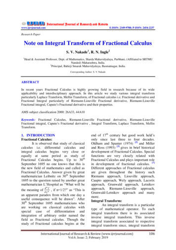
Example 6.3 (p.173)Perform the Laplace transforms on (a) step function u0(t), and (b) ua(t) in the following two figures:Step function ua(t):Step function u0(t):f(t)f(t)11t00taSolution:(A) Laplace transform of function u0(t):We learned from Chapter 2 that both ramp and step functions provide math expressionsfor physical phenomena that begin to exist at t a in the function illustrated in Example 6.2,and t 0 for the step function u0(t) at t 0, and ua(t) at t a in the above figures. Laplacetransforms for both these step functions in this example may be obtained as:We have the Laplace transform of this function using in integral in Equation (6.1) or as includedin Case 1 in Appendix 1 to be:L u 0 (t ) 0(1) e st1dt e sts 01s8
(B) Laplace transform of function ua(t):f(t)The mathematical expression of function f(t) inthis case is available in Equation (2.36a) (p.58)with α 1, that is: f (t ) u a (t ) 10ta0 t aa t 01The corresponding Laplace transform is:L u a (t ) a0(0) e st dt (1) ea st1dt e sts a1 asesWe will find that the result of the step function ua(t) as shown above is identical to thatshown in Case 15 in the Laplace Transform Table in Appendix 1.9
6.3Properties of Laplace Transform (p.174)Laplace transform of functions by integration:Lt f t 0e st f t dt F s (6.1)is not always easy to determine.Laplace transform (LT) Table in Appendix 1 is useful, but does not always have therequired answer for the specific functions. Following properties are selected for the LTof some functions:6.3.1. Linear operators:L[a f(t) b g(t)] a L[f(t)] b L[g(t)](6.5)where a, b constant coefficientsExample 6.4:Find Laplace transform of function: f(t) 4t2 – 3Cos t 5e-t with 0 t :Solution:By using the linear operator, we may break up the transform of f(t) into three individualtransformations:L(4t2 – 3Cos t 5e-t) 4L[t2] – 3L[Cos t] 5L[e-t] F(s)Case 3 with n 3HenceCase 18 with ω 1F (s) Case 7 with a -1 from the LT Table83s5 s3 s2 1 s 110
Properties of Laplace Transform – Cont’d6.3.2. Shifting property (p.175):If the Laplace transform of a function f(t) is L[f(t)] F(s) by integration, or fromthe Laplace Transform (LT) Table, the Laplace transform of G(t) eatf(t) can beobtained by the following relationship:L[G(t)] L[eatf(t)] F(s-a)(6.6)where a in the above formulation is the shifting factor, i.e. the parameter s inthe transformed function f(t) that has been shifted by (s-a)Example 6.5:Perform the Laplace transform on function: F(t) e2t Sin(at), where a constantSolution:We may either use the Laplace integral transform in Equation (6.1) to get the solution, orwe could get the solution available the LT Table in Appendix 1 with the shifting property forthe solution. We will use the latter method in this example, with:L[ f (t )] L[ Sin at ] as a22(Case 17 in Appendix 1),The Laplace transform of F(t) e2tsin(at) can thus be obtained by using the shift amount of2 in Equation (6.6), or in the form:aL[ F (t )] L[e 2t Sin at ] ( s 2) 2 a 211
6.3.3. Change of scale property (p.175):If we know L[f(t)] F(s) either from the LT Table, or by integral in Equation (6.1),we may find the Laplace transform of function f(at) by the following expression:1 s F a a where a scale factor for the changeL[ f (at )] (6.7)Example 6.6:Perform the Laplace transform of function F(t) sin3t.Since we know the Laplace transform of f(t) sint from the LT Table in Appendix 1 as:L[ f (t )] L[ Sint ] 1 F (s)s2 1We may find the Laplace transform of F(t) using the “Change scale property” withscale factor a 3 to take a form:L[ Sin 3t ] 113 3 s 2s2 9 1 3 12
6.4Inverse Laplace Transform (p.176)We have defined the Laplace transform of a function f(t) to be:Laplace transformFrom hereLt f t 0to theree st f t dt F s (6.1)there are times we need to do the following:Lt f t to there 0e st f t dt F s From hereInverse Laplace transformThere are 4 available ways to inverse Laplace transforms to engineers: Use LT Table by looking at F(s) in right column for corresponding f(t) in middle column- the chance of success is not very good. Use partial fraction method for F(s) rational function (i.e. fraction functionsinvolving polynomials), and The convolution theorem involving integrations. Use the Bromwich contour integrations around residues in the approximate form of F(s)using complex variable theories. This method will not be presented in this class13because it is beyond the scope of this course.
6.4.2The Partial Fraction Method for Inverse Laplace Transform (p. 176) The expression of F(s) to be inversed in Laplace transform is expressed in the followingpartial fractions:P( s)F (s) Q( s)where polynomial P(s) is at least one order less than the order of polynomial Q(s) “Break” up the above rational function into summation of “simple fractions”:F ( s) AnA1A2P( s) . Q( s) s a1 s a 2s an(6.8)where A1,. A2, .An, and a1, a2, .an are constants to be determined bycomparing coefficients of terms on both sides of the equality:AnP( s)A1A2 . Q( s) s a1 s a2s an The inverse Laplace transform of F(s) P(s)/Q(s) becomes:a fraction a sum of partial fractions14
Example 6.7 (p.177):Perform the inverse Laplace transform of the following expression:F (s) Solution:3s 7P s 2Q s s 2 s 3We may express F(s) in the following partial fraction form:F (s) ABA s 1 B s 3 3s 73s 7 s 3 s 1 s 2 2 s 3 ( s 3)( s 1) s 3 s 1where A and B are constant coefficientsAfter expanding the above rational function and equating the terms in the numeratorsof both sides of the above equality:3s 7 A(s 1) B(s-3) (A B)s (A – 3B)We may solve for A and B from the above simultaneous equations:A 4 and B -1A B 3and A – 3B 7 resulting in:We will thus have:3s 741 s 2 2s 3 s 3 s 1The required Laplace transform is: 3s 7 1 1 1 1 3t t L 1 4LL 4e e s 3 s 1 ( s 3)( s 1) 15
Example 6.8:Perform the following inverse Laplace transform:Solution: P s 3s 1 1 L 1 F ( s ) L 1 L s 3 s 2 s 1 Q s We may break up F(s) in the above expression in the following form:P s Q s 3s 1ABs C ( s 1)( s 2 1) s 1s2 1The polynomial in numeratoris always one order less thanthat in the denominatorBy following the same procedure, we determine the coefficients A 2, B -2 and C 1, or:3s 122s1 ( s 1)( s 2 1) s 1s2 1 s2 1We will thus have the inversed Laplace transform, and thus the original function f(t) to be:3s 11 1 2 1 2 s 1 tf (t ) L 1 F ( s ) L 1 3LLL 2e 2 Cos t Sin t 222 s 1 s 1 s s s 1 s 1 16
6.4.3Inverse Laplace Transform by Convolution Theorem(p.178) This method involves the use of integration of the expressions involving LT parameter s - F(s) There is no restriction on the form of the expression F(s): – they can be rational functions ofpolynomial, trigonometric functions or exponential functions The convolution theorem works in the following ways for inverse Laplace transforms:If we know the following:L-1[F(s)] f(t) andL-1[G(s)] g(t), with: F ( s ) 0 e st f (t ) dt , and G ( s) e st g (t ) dt0from the LT Table in Appendix 1 or using integration in Equation (6.1), then the desiredinverse Laplace transform of Q(s) F(s) or G(s) can be obtained by:the following integrals:Either by: L 1Or by: Q(s) L F (s)G(s) 0 1L Q( s) L F ( s)G ( s) 1 1tf ( ) g (t ) d t0f (t ) g ( ) d (6.9a)(6.9b)17
Example 6.9 (p. 178):Find the inverse of a Laplace transformed function with: Q( s ) ss2 a2 2Solution:We may express F(s) Q(s) in the following expression:(a)It is our choice to select F(s) and G(s) in the above expression for the integrals inEquation (6.9a) or (6.9b).s1 andGsF s 2 Let us choose:s a2s2 a2From the LT Table in Appendix 1, we get the following:L 1 F s Cos at f t and L 1 G s Sin at g t aThe inverse of Q(s) F(s)G(s) is obtained by Equation (6.9a) as: sL 1 s 2 a 2 Sin a(t )t Sin att Cosad 02a2a One will get the same result by using another convolution integral in Equation (6.9b), orusing partial fraction method in Equation (6.8)18
Example 6.11 (p.179):Use convolution theorem to find the inverse Laplace transform: Q ( s ) Solution:We may express Q(s) in the following form:Q( s) 1( s 1)( s 2 4)111 ( s 1)( s 2 4) s 1 s 2 4(a)We choose F(s) and G(s) as:F (s) 1or e t f t s 1andG (s) 11orSin 2t g t s2 42Let us use Equation (6.9b) for the inverse of Q(s) in Equation (a):q (t ) t0f (t ) g ( ) d t01 1 e ( t ) Sin 2 d e t2 2 t0e Sin 2 d After the integration , we get the inverse of Laplace transform Q(s) to be:q (t ) 1 t11 t e Sin 2 2 Cos 2 1e Sint Cost e22 2552 1 2 0 10 t19
6.5Laplace Transform of Derivatives (p.180) We have learned the Laplace transform of function f(t) by:Lt f t 0e st f t dt F s We realize the derivative of function f(t):f ' (t ) (6.1)df (t )is also a FUNCTIONdtSo, there should be a possible way to perform the Laplace transform of the derivativesas functions, as long as its variable varies from zero to infinity. Laplace transform of derivatives is necessary steps in solving DEs using Laplace transform By following the mathematical expression for Laplace transform of functions in Equation (6.1),we may expression Laplace transform of derivative f’(t) in the following form:L f ' (t ) 0e st f ' (t ) dt We will use “integration by parts” techniqueFor this integral by letting:We will further assign:u e stdu se st dtand 0 df (t ) e st dt dt 0udv uv df t dv dt (6.10) 0 vdu0v f(t)20
By substituting the above ‘u’, “du”, “dv” and “v” into the following relationship:L f ' (t ) 0e st f ' (t ) dt df (t ) dte st dt 0 0We will have:L f ' (t ) 0e st f ' (t ) dt udv uv 0 vdu0 df (t ) st ste st dt ef(t) f(t) sedt 00 dt 0(6.11), leading to:L f ' (t ) 0 00e st f ' (t ) dt e st f (t ) or in a simplified form: f (t ) se st dt f (0) s e st f (t )dt f (0) sL f (t ) L[f’(t)] s L[f(t)] – f(0) 0(6.12) Likewise, we may find the Laplace transform of second order derivative of function f(t) to be:L[f’’(t)] s2 L[f(t)] – sf(0) – f’(0)(6.13) A recurrence relation for Laplace transform of higher order (n) derivatives of function f(t)may be expressed as:(6.14)L[fn(t)] snL[f(t)] - sn-1 f(0) – sn-2f’(0) – sn-3f’’(0) - .fn-1(0)21
Example 6.12 (p.181):Find the Laplace transform of the second order derivative of function: f(t) t SintThe second order derivative of f(t) meaning n 2 in Equation (6.14), or as inEquation (6.13):L[f’’(t)] s2 L[f(t)] – sf(0) – f’(0)We thus have: d 2 f t 2' 0 L sLft sf0 f 2dt f ' t Since(6.13)df t d t Sin t t Cos t Sin tdtdtWe thus have:L f " (t ) s 2 L f (t ) s f (0) f ' (0) s 2 L t Sin t s(t Sin t ) t 0 (t Cos t Sin t ) t 0 s 2 L t Sin t 22
6.5.2 LaplaceTransform of Partial Derivatives (p.181)In Section 2.2.5 (p.36), we learned that partial derivatives involving more than oneindependent variable in the function and they appear frequently in engineering analyses. It isnecessary for engineers to learn how to perform Laplace transform of these functions and theirderivatives.Functions involving more than one independent variable in forms such as: f(x,t), f(x,y,t) orf(x,y,z,t), in which x, y, z and t are independent variables - with (x,y,z) represent variables inspace and t for the time.Laplace transform can be performed on partial derivatives, BUT with one variable ata time ONLY, as long as the variable to be transformed satisfy the condition of:0 (variable) Let us elaborate the above statement by an example for a function f(x,t) with a space variable xand another independent variable time t.The rate of change of the values of this function f(x,t) depends on both values of these twoindependent variables –x and t, or mathematically to be expressed as: f x, t for the rate of change of function f(x,t) with respect to variable x, and x f x, t for the rate of change of function f(x,t) with respect to the other variable t, t2 2 f x, t are the corresponding second order partial derivatives of the f x , t andfunction f(x,t) t 2 x 223
6.5.2Laplace Transform of Partial Derivatives – Cont’dLet us designate the Laplace transform of a function with two independent variables x and t by:L x f x, t 0e sx f x, t dx F* s, t with 0 x (6.15)to be the Laplace transform of function f(x,t) with respect to variable x, andL t f x, t 0e st f x, t dt F* x, s with 0 t (6.16)to be the Laplace transform of function f(x,t) with respect to the variable t.The subscripts attached to the Laplace transform operator (L) in Equations (6.15) and (6.16)denotes the variable to be transformed by the Laplace transform.We were reminded again and again that function this is qualified for Laplace transform mustsatisfy the condition that the variable to be transformed must satisfy the condition:0 (variable) .Let us assume that of the two independent variable x and t involved in the function f(x,t), butonly the variable t satisfies this condition 0 t , (the other variable x does not satisfythis condition). We can thus only have Laplace transform on the variable t in this case.Consequently, we will have the following Laplace transform of the function f(x,t): f x , t Lt x 0 st F* x , s f x , t e dt e f x , t dt x 0 x x st(6.17)24
6.5.2 LaplaceTransform of Partial Derivatives – Cont’dThe expression of Laplace transform of the partial derivative of function f(x,t):is not straightforward as one would imagine. The following steps need to be taken to get theappropriate expression for this partial derivative. Let us follow what we did in thecase for functions with single variable in Section 6.5.1, with the following integration:I 0 f x , t e st dt t 0 udv uv 0 vdu in which u and v are parts of the integral (I).0If we let u e-st leading to du -se-stdt, and dv Resulting in: f x, t dt leading to v f(x,t). t f x, t st st Lt I efx,t sef x, t dt t 0 0t f x,0 s e st f x, t dt f x,0 sF * x, s (6.19)0We may thus express the Laplace transform of partial derivatives in the following expressionfor the Laplace transform of the partial derivative as: f x, t * x , s f x ,0 Lt sF t (6.20)Likewise, we may show that the Laplace transform of second order partial derivatives as follows: 2 f x, t f x , t 2 f x , t 2 F * x, s 2**Lt and Lx (6.21a,b) s F x, s sF x , s t2 22 t xt 0 x 25
Example 6.13 (p.183)If the Laplace transform of the function θ(x,t) xe-t is defined as:Lt x, t * x, s and with: 0 t Determine: x, t (a ) Lt x b 0e st x, t dt x, t Lt 2 x 2 c (a) x, t Lt t d 2 x, t Lt 2 t Solution:We first establish the Laplace transform of the multi-variable function θ(x,t) xe-t byusing Equation (a) and obtain: Lt x, t x Lt e t x * x, s s 1We will then proceed to determine the four required Laplace transforms of the derivatives offunction θ(x,t) as required by using Equations (6.21 a,b).* x 1 x, t ( x, s) a Lt x x s 1 s 1 x b 2 x, t 2 * x, s 1 0 Lt 22 1 xxxs sxx x, t * sxsxx (c) Lt , ,0 s 1s 1 t d 2 x , t x , t s2x2*Lt sx x s x , t s x ,0 2 t ts 1 t 02s xx sx x s 1s 126
6.6Solution of Differential Equations Using Laplace Transforms (p.184) One popular application of Laplace transform is solving differential equations However, such application MUST satisfy the following two conditions:(1) The variable(s) in the function for the solution, e.g., x, y, z, t must coverthe range of (0, ).It means that the solution, e.g., u(x) or u(t) MUST also be VALIDfor the range of (0, ), and(2) ALL appropriate conditions for the differential equation MUST be available with theproblem The solution procedure is presented below:(1) Apply Laplace transform on EVERY term in the differential equation (DE)(2) The Laplace transform of derivatives results in given conditions, such as f(0),f’(0), f”(0), etc. as shown in Equation (6.14)(3) After apply the given values of the given conditions as required in Step (2),we will get an ALGEBRAIC equation for F(s) as defined in Equation (6.1):L f t 0e st f t dt F s (6.1)(4) We thus can obtain an expression for F(s) from Step (3)(5) The solution of the DE is the inverse of the Laplace transformed F(s), i.e.,:y(t) L-1[F(s)]27
Example 6.14 (p.184):Solve the following DE with given conditions:d 2 y (t )dy (t ) t 2 5y(t) eSin t2dtdtgiven conditions:y(0) 0and0 t (a)(b)y’(0) 1Solution:(1) Apply Laplace transform to EVERY term in the DE in Equation (a): d 2 y (t ) dy (t ) t 25()L L Lyt LeSin t 2 dt dt whereL y (t ) 0 (c)y (t ) e st dt Y ( s )Equations (6.12) and (6.13) for the Laplace transforms of the first and second orderderivatives in Equation (c) will result in: s2 Y ( s ) sy (0) y ' (0) 2 sY ( s ) y (0) 5 Y ( s ) 11 ( s 1) 2 1 s 2 2 s 2(d)(2) Apply the given conditions in Equation (b) in Equation (d): s 02 1 0Y ( s ) sy (0) y ' (0) 2 sY ( s ) y (0) 5 Y ( s ) 11 ( s 1) 2 1 s 2 2 s 228
(3) We can obtain the expression:s 2 2s 3Y (s) 2s 2s 2 s 2 2s 5 (e)(4) The solution of the DE in Equation (a) will be obtained by the inverse Laplace transformof Y(s) in Equation (e), i.e. y(t) L-1[Y(s)], or: s 2 2s 3y t L Y s L 2 2s2s2s2s5 1 1 (5) The inverse Laplace transform of Y(s) in Equation (e) is obtained by using either“partial fraction method” or “convolution theorem.” The expression of Y(s) can beshown in the following form by “partial fractions:”121121Y (s) 2 3 2 3 2 23 s 2s 2 3 s 2s 5s 2s 2 s 2s 5The inversion of Y(s) in the above form is:y (t ) L 1 [Y ( s )] 1 1 12 1 112 1 1 1 1 L 2LLL 222 s 2s 5 33 s 2s 2 33 ( s 1) 4 ( s 1) 1 Leading to the solution of the DE in Equation (a) to be:y (t ) L 1 Y ( s ) 1 t2 1 t1e Sin t e Sin 2t e t Sin t Sin 2t 33 2329
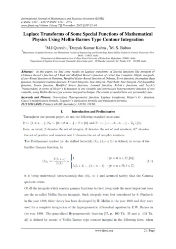
6.6 Solution of Differential Equations Using Laplace Transforms-Cont’d6.6.2 Differential equations for the bending of beams (p.186):We offer this method for solving problems of indeterminate beam bending (the cases inwhich the number of unknowns in the mechanic analysis of beams subject to bending loadsexceed the total number of end conditions that engineers can derive from the static equilibriumconditions).Laplace transform method is found to be effective in solving problems of beam bendingof this kind. The following figure illustrates the different situations of statically determinateand statically indeterminate beams; we notice the loaded beam in the left involves 2 unknownsof reactions at supports A and B which can be determined by the two available end conditionsfrom free-body force diagram. The similar situation is illustrated in the right of the diagram, in which we realize that it has three (3) unknowns involving two reactions RA and RB at thesupports A and B and the bending moment MA in Support A. These three unknownscannot be solved with the available two (2) conditions by the Supports A and B. This situationis termed as “indeterminate.” Solutions to indeterminate beam bending are usually tedious andcumbersome. We will demonstrate the use of Laplace transform technique involving specialfunctions to be an effective alternative solution method for the solution of bending ofindeterminate beams subjected to loading to parts of the beams.Statically determinate beam with 2 unknowns:AStatically indeterminate beam with 3 unknowns:P 5000 lbfBMARARBAP 5000 lbfB RAFigure 1.10 Static bending of beamsRB30
6.6Solution of Differential Equations Using Laplace Transforms-Cont’d6.6.2 Differential equations for the bending of beams-Cont’d (p.186):We may derive a differential equation from the theory of elasticity to determine thedeflection of a beam y(x) induced by a distributed bending load W(x) per unit length asillustrated in the figure below:The induced deflection in the beam y(x) at location x can be obtained by solving theEuler-Bernoulli equation in the following differential equation:d 4 y x W ( x) 4EIdx(6.22)where E is the Young’s modulus of the beam material and I is the section moment ofinertia of the beam cross-section.The product of EI is referred to as the flexural rigidity of the beam structure.31
6.6 Solution of Differential Equations Using Laplace Transforms-Cont’d6.6.2 Differential equations for the bending of beams – cont’d:Example 6.15 (p.187):Use the Laplace transform method to find the induced deflection function y(x) of a cantileverbeam by a uniform distributed load with intensity w0 on half of the beam span as illustrated inFigure 6.5.Figure 6.5 A Cantilever beam subjected to uniform distributed loadThe beam subjected to bending as illustrated in Figure 6.5 would be difficult to solve for it’sinduced deflection and the bending stress by traditional simple beam theory because it is astatically indeterminate beam bending problem. Laplace transform method combined with astep function for the loading situation is a viable alternative method in solving this problem.One critical issue, however, is that one must bear in mind that Laplace transform can onlybe used in the situation that the variable to be transformed must satisfy the condition of:0 (variable) 32
6.6 Solution of Differential Equations Using Laplace Transforms-Cont’d6.6.2 Solving differential equations for the bending of beams using Laplace Transform– cont’d (p.187):The DE:d 4 y x W ( x) dx4EI(a1)The applied loading function W(x):W(x) W0 for 0 x L/2 0for L/2 x LWe thus have the differential equation for the solution with the form:d 4 y x W0with 0 x L/2 dx 4EI 0(a2)with L/2 x Lwith the following end (or boundary) conditions:At x 0:At L:y x x 0 y 0 0(zero deflection)(b1)dy x y ' 0 0dx x 0(zero slope for the “built-in end support)(b2)d 2 y x y ' ' L 0dx 2 x L(zero bending moment at free-end)d 3 y x y ' ' ' L 0dx 3 x L(zero shear force at free-end)(b3)(b4)33
6.6 Solution of Differential Equations Using Laplace Transforms-Cont’d6.6.2 Solving differential equations for the bending of beams using Laplace Transform– cont’d (p.188):We notice that the variable x that is associated with the deflection function y(x) in theproblem covers a finite range with 0 x L. The legitimacy of using the Laplace transformmethod in solving the differential equation requires the expression of this function y(x) withits variable x covering the spectrum of (0, ).We thus need to derive the form of Equation (a1) from the variable range (0.L) to thedomain (0, ) in order to use the Laplace transform method for solving Equation (a1).By using the definition of step functions in Section 2.4.2, we may convert the currentloading function W(x) from the spectrum of (0,L) to (0, ):W(x) W0[u(x) –u(x-L/2)] with 0 x (c)where u(x) is the unit step function as defined in Section 2.4.2 (p.58), and with its shapeillustrated in Figure 2.51 on p.60.The equation for the deflection function y(x) in Equation (a1) will thus become:d 4 y x W0 L uxux EI 2 dx 4 with 0 x ,(a3)We may thus use the Laplace transform method to solve the deflection function y(x) inEquation (a3) togather with the end conditions in Equations (b1) to (b4). Let Y(s) to bethe function y(x) after the Laplace transform with the following definition of Y(s):L f ( x) 0e sx f x dx Y ( s)(d)34
6.6 Solution of Differential Equations Using Laplace Transforms-Cont’d6.6.2 Solving differential equations for the bending of beams using Laplace Transform– cont’d:Upon applying the Laplace transform in Equation (d) to the differential equation in (a3), we willsLge
Laplace Transform in Engineering Analysis Laplace transform is a mathematical operation that is used to "transform" a variable (such as x, or y, or z in space, or at time t)to a parameter (s) - a "constant" under certain conditions. It transforms ONE variable at a time. Mathematically, it can be expressed as: