Transcription
AIRBORNE LIDAR BATHYMETRY BEAM DIAGNOSTICS USING AN UNDERWATEROPTICAL DETECTOR ARRAYBYMATTHEW BIRKEBAKBSME, University of New Hampshire, 2015THESISSubmitted to the University of New Hampshirein Partial Fulfillment ofthe Requirements for the Degree ofMaster of ScienceinOcean Engineering: Ocean MappingMay, 2017
This thesis has been examined and approved in partial fulfillment of the requirements for thedegree of Masters of Science in Ocean Engineering: Ocean Mapping by:Thesis Director, Dr. Shachak Pe’eri, Research AssociateProfessor, Center for Coastal and Ocean MappingDr. Firat Eren, Research Scientist, Center for Coastal andOcean MappingDr. Neil Weston, Technical Director, National Oceanic andAtmospheric Administration, Office of Coast SurveyOn April 6th, 2017Original approval signatures are on file with the University of New Hampshire Graduate School.ii
ACKNOWLEDGEMENTSThis work was possible through the help of many of my advisors and mentors. I would like tothank professors Shachak Pe’eri, Firat Eren and Neil Weston who dedicated time and effort intothis project. Also very special thanks to Paul Lavoie for his enormous help in the construction ofthe detector array and waterproof housings. I would also like to thank Dr. Yuri Rzhanov for hishelp with the image processing, Carlo Lanzoni for his help producing the detector array circuitryand Sean Kelley for his work on the data collection and analysis.Finally I thank the National Oceanic and Atmospheric Administration for their support and fundingthat made this research possible.Joint Hydrographic Center / Center for Coastal and Ocean Mapping (NOAA Ref. No:NA15NOS4000200)iii
TABLE OF CONTENTSACKNOWLEDGEMENTS . iiiTABLE OF CONTENTS . ivLIST OF FIGURES . viiLIST OF TABLES . xiiABSTRACT . xiv1.INTRODUCTION . 12.RAY-PATH GEOMETRY . 83.4.2.1Transmission from the ALB System . 92.2Interaction of the ALB Beam with the Water Surface . 112.3Total Propagated Uncertainty (TPU) of ALB Depth Measurements . 14WATER SURFACE CHARACTERISTICS . 183.1Linear Wave Theory. 203.2Beam Interaction with Water Surface . 223.3Elevation Models for Water Surfaces . 24METHODOLOGY . 314.1Ray Tracing Models . 324.2Empirical Laser Beam Diagnostics . 384.3Experimental Setup and Incident Angle Calibration. 42iv
5.6.7.RESULTS . 465.1Wind Wave Measurements . 465.2Ray Tracing Results . 515.3Detector Array Results . 565.4Sub Surface Refraction Angle Deviation . 605.5Beam Footprint Analysis . 635.6Uncertainty Model. 71DISCUSSION . 736.1Uncertainty Model. 736.2Future Work . 75CONCLUSIONS. 77REFERENCES . 79APPENDIX . 84A. Wave Spectrum Models . 84JONSWAP Spectrum (Used for Apel calculations) . 84Apel spectrum (1994) . 84B. Optical Detector Array . 86Photodiodes . 86Waterproof Housing. 88v
Mounting Grid . 89C. Photodiode Calibration . 91Responsivity. 91Temperature Sensitivity . 93Thermal Time Constant . 95Thermal Temperature Dependence . 97Field of View . 99D. Image Processing Techniques . 100Image Moment Invariants . 100Centroid Analysis. 101E. Additional Centroid Analysis Datasets . 102vi
LIST OF FIGURESFigure 1.1: Example ALB waveform consists of three parts: the surface reflection, volumebackscatter, and the bottom reflection. Image from Guenther (2007). . 1Figure 2.1: Basic ray path geometry of ALB beam refracting into water. . 8Figure 2.2: Beam properties near water surface. . 10Figure 2.3: Example of a Gaussian (TEM 00) beam intensity distribution. . 11Figure 2.4: Snell's Law . 12Figure 2.5: Geometric stretch of laser beam on the water surface. . 14Figure 2.6: An illustration of the effect of slant path error as depicted by Karlsson, 2011. The errorin refraction angle causes a horizontal error (ΔX) and a vertical error (ΔZ). . 17Figure 3.1: The Beaufort wind scale. ALB surveys are limited to conditions less than Beaufortscale 3. Encyclopedia Britannica (2009). . 19Figure 3.2: A progressive wave modeled by Airy wave theory. Image from Dean and Dalrymple(1984). . 20Figure 3.3: A surface composed of several waves (a) can be separated in to the individualmonochromatic elements (b). 22Figure 3.4: Altered slant path of laser beam due to variation in water surface slope causes a verticaland horizontal error in the measurement. Most ALB systems have no correction for this error. 24Figure 3.5: Four monochromatic waves of different size and propagating in different directionssuperimpose to form a complex water surface. . 25vii
Figure 3.6: Example Apel wave spectra with very short fetches to simulate experimentalconditions. U10 5m/s. . 27Figure 3.7: Wave spreading function based on the cosine squared model. Larger values of scorrespond to longer gravity waves. . 28Figure 3.8: Wave spectrum, spreading function, and directional spectrum for an Apel wavespectrum model with U 5m/s, fetch 5m. . 29Figure 3.9: a) The two sided wave spectrum. b) The real Hermitian amplitudes. c) The imaginaryHermitian amplitudes. d) The water surface realization for a small patch of water (0.5 m x 0.5 m). 30Figure 4.1: A magnified surface triangulated using Delaunay triangulation. The Apel spectrum fora fetch of 7.5m and wind speed of 5kts was used to find the surface elevation points. . 33Figure 4.2: a) The simulation of 10,000 rays incident on the water surface model. In this case thebeam is at a 20 incidence angle to the horizontal. b) the beam footprint on the water surface withGaussian ray distribution . 34Figure 4.3: Rays refracting through the numeric surface, each ray was mapped to a depth of 0.25cm. 35Figure 4.4: Sub surface beam footprint as predicted by the model. 1000 rays with a 0.1m beamdiameter (FWHM) at water surface, θi 20 . . 36Figure 4.5: Model results for U 5.25 m/s, θ 15 . The blue stars represent the center ofconcentration of each unique beam that was analyzed, the red star is the mean of these results. Theorigin of the plot represents the still water center of concentration. . 37viii
Figure 4.6: Optical detector array with acrylic waterproof housings. . 39Figure 4.7: Experimental setup in the Chase Ocean Engineering Wave and Tow Tank, used forangle of incidence estimation. 40Figure 4.8: Example of raw pixel bit value related to the intensity of the laser beam. This imageshow the footprint of the 20cm diameter laser beam just below a still surface. . 41Figure 4.9: Disturbed water surface experiments. a) The fan generates surface waves that interactwith the laser beam that is projected on the array. b) A subsurface view of a turbulent laser beamon the array. . 43Figure 4.10: Incidence angle calibration setup. The laser was moved horizontally along x withchanging angle θ to provide the correct angle of incidence on the water surface. The refractionangle was then calculated for use with array calibration. . 44Figure 4.11: Image moment values versus the incident angle. M13 shows a strong correlation. 45Figure 4.12: The calibration curve for the M13 vs. incidence angle. This correlation provides thein air estimation of incidence angle for any unknown footprint. . 45Figure 5.1: a) The velocity output of the l fan is seen to have spherical spreading ( r -2) withdistance downwind. b) Over the range of distances studied, the fan output changes by less than1m/s. . 46Figure 5.2: Water surface elevation at 3.5m from fan. . 47Figure 5.3: The wave spectrum and Apel model spectrum for each distance from the fan. Windspeed measured with the anemometer was used for the spectrum model. . 48ix
Figure 5.4: Wave spectrum at each distance downwind. The frequency contend in the 6-10 Hzrange is similar in each case. 49Figure 5.5: Experimental spectrum matched to fully developed gravity-capillary Apel 1994 (fetchof 30m) wave spectrum. . 50Figure 5.6: The standard deviation values in the along wind direction from each simulationcomparing incidence angle and wind speed. The beam diameter for all simulations was D 0.25m. 52Figure 5.7: Refraction angle deviation averaged over incidence angle (D 0.25m). . 53Figure 5.8: For U 2.5 m/s and D 0.25m, the relationship between beam refraction error and stillwater incidence angle. . 53Figure 5.9: θ 15 for all simulations. The larger diameter beams are effected less by the surfaceripples than beams with diameters less than 1m. . 54Figure 5.10: The surface error decays exponentially with laser beam diameter. . 55Figure 5.11: θ 0 , still water surface. Near Gaussian intensity distribution. Pixels are labeled onX and Y axis. 56Figure 5.12: θ 20 , still water surface. At higher incidence angle a more elliptic beam shape. Pixelsare labeled on X and Y axis. . 57Figure 5.13: θ 0 , U 2m/s. A sample of detector array intensity readings in a disturbed surfacecase. . 58Figure 5.14: θ 20 , U 4m/s. A sample of detector array intensity readings in a disturbed surfacecase. . 59x
Figure 5.15: Short samples of sub surface estimated incidence angle curves at a 10 still waterincidence. . 61Figure 5.16: The centroid results at distances of 3.5 to 7.5 m from the fan at an incidence angle of0 . . 64Figure 5.17: The centroid results at distances of 3.5 to 7.5 m from the fan at an incidence angle of15 . . 65Figure 5.18: Along wind standard deviation of beam center as a function of distance. . 66Figure 5.19: The refraction angle deviation is seen to clearly increase with wind speed in bothalong and cross wind directions. . 67Figure 5.20: The along wind refraction angle deviation increases with incidence angle while thecross wind error decreases. . 68Figure 5.21: Beam footprint analysis for still water case with in air incidence angle of 15 . . 69Figure 5.22: Beam footprint analysis for a wave refracted footprint. The contour line is irregularand there is an increase in beam diameter from the still water case. . 70Figure A.1: Example Apel spectrum for fetch 30 m and U 5 m/s. . 85Figure B.1: The reverse bias circuit to be used with photodiodes as provided by ThorLabs. . 86Figure B.2: ThorLabs PD1A Photodiode (www.thorlabs.com) . 88Figure B.3: Waterproof housing for photodiode. 89Figure B.4: Mounting Grid . 90Figure B.5: Array mounted to frame. 90xi
Figure C.1: ND:YAG laser power vs. dial setting . 92Figure C.2: Photodiode output vs. laser power . 93Figure C.3: Temperature effect on QE vs Wavelength (3. Quantum Efficiency) . 95Figure C.4: Thermal Time Constant for Housing. . 96Figure C.5: Thermal Dependence . 97Figure C.6: Example of FOV crosstalk. 99Figure E.1: The centroid results at distances of 3.5 to 7.5 m from the fan at an incidence angle of10 . . 102Figure E.2: The centroid results at distances of 3.5 to 7.5 m from the fan at an incidence angle of20 . . 103LIST OF TABLESTable 1.1: ALB system specifications according to manufacturers (Quadros N. , 2013). . 2Table 5.1: Spectrum peak and significant wave height for wind ripples present in lab experiments. 49Table 5.2: Fan generated tank conditions and the estimated real world survey wind conditions. 51Table 5.3: 2σ Refraction angle deviations ( ) from the image moment calculations. . 62Table 5.4: Trend line values for the beam refraction angle deviation results. . 66Table 5.5: Refraction angle uncertainty in along wind axis. . 72Table 5.6: Refraction angle uncertainty in cross wind axis. . 72xii
Table 6.1: Uncertainty values for ALB systems reported as 2σ standard deviations. . 74Table C.2: Field of View Results. 100xiii
ABSTRACTAIRBORNE LIDAR BATHYMETRY BEAM DIAGNOSTICS USING AN UNDERWATEROPTICAL DETECTOR ARRAYbyMatthew BirkebakUniversity of New Hampshire, May, 2017The surface geometry of air-water interface is considered as an important factor affecting theperformance of Airborne Lidar Bathymetry (ALB), and laser optical communication through thewater surface. ALB is a remote sensing technique that utilizes a pulsed green (532 nm) lasermounted to an airborne platform in order to measure water depth. The water surface (i.e., air-waterinterface) can distort the light beam’s ray-path geometry and add uncertainty to range calculationmeasurements. Previous studies on light refracting through a complex water surface are heavilydependent on theoretical models and simulations. In addition, only very limited work has beenconducted to validate these theoretical models using experiments under well-controlled laboratoryconditions.The goal of the study is to establish a clear relationship between water-surface conditions and theuncertainty of ALB measurement. This relationship will be determined by conducting moreextensive empirical measurements to characterize the changes in beam slant path associated witha variety of short wavelength wind ripples, typically seen in ALB survey conditions. This studyxiv
will focus on the effects of capillary and gravity-capillary waves with surface wavelengths smallerthan the diameter of the laser beam on the water surface. Simulations using Monte-Carlotechniques of the ALB beam footprints and the environmental conditions were used to analyze theray-path geometries. Based on the simulation results, laboratory experiments were then designedto test key parameters that have the greatest contribution on beam path and direction through thewater. The laser beam dispersion experiments were conducted in well-controlled laboratory settingat the University of New Hampshire’s Wave and Tow tank.The spatial elevations of the water surface were independently measured using a high resolutionwave staff. The refracted laser beam footprint was measured using an underwater optical detectorconsisting of a 6x6 array of photodiodes. Image processing techniques were used to estimate thelaser’s incidence angle intercepted by the detector array. Beam patterns that resulted fromintersection between the laser beam light field underwater and the detector array were modeledand used to calculate changes in position and orientation for water surface conditions containingwavelengths less than 0.1m. Finally, a total horizontal uncertainty (THU) model was estimated,which can be implemented in total propagated uncertainty (TPU) models for reporting as ameasure of the quality of each measurement. The wave refraction error for various sea states andbeam characteristics was successfully quantified using both experimental and analyticaltechniques.xv
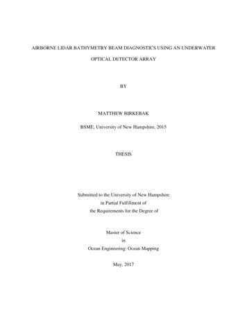
1. INTRODUCTIONAirborne Lidar Bathymetry (ALB) is a coastal survey system that measures water depth using apulsed scanning laser mounted to an airborne platform. Common ALB laser pulses aretransmitted at a green wavelength that is generated by frequency doubling of the fundamentalwavelength Nd:YAG laser from 1064 nm to 532 nm (Guenther et al., 1994; Penny, et al., 1986).The choice of a green wavelength is because of the ocean’s optical characteristics, in which theminimum spectral absorption for most waters is at green wavelengths (Jerlov, 1968). Theinteractions of the laser pulse with the environment is typically logged over time as a waveform(Figure 1.1). Water depth is calculated using the Time of Flight (TOF) between the laser pulseinteractions with the water surface (surface return) and seafloor (bottom return). In order tocalculate the position of the laser beam on the seafloor for depth and position reporting, it isimportant that the refracted beam path of the laser is known including aircraft attitude andmotion corrections (Guenther, 1985).Figure 1.1: Example ALB waveform consists of three parts: the surface reflection, volume backscatter, and the bottomreflection. Image from Guenther (2007).1
Standard operating conditions for commercial ALB data collection are typically at altitudesranging from 300 to 600 m above the water surface. Although various ALB systems may vary inhardware specifications (Table 1.1), the ray-path geometry of the laser beam in all systems is thesame. The ALB’s ray-path geometry includes a transmission of a laser beam with a typical solidangle of 5 to 45 mrad. The laser beam propagates through the atmosphere then interacts with thewater surface. A small part of the laser energy is scattered at the water surface and reflects backto ALB detector, while most of the laser energy propagates down the water column. Within thewater column, the laser beam may interact with suspended and dissolved material (i.e., additionalscattering) until it intersects with the bottom. The reflection pattern of the laser beam back up thewater column will depend on seafloor characteristics including slope and roughness. It isassumed that the returning ray-path of the laser beam is near identical to the transmit pathfollowing Green’s reciprocity principle (Guenther, 1985). The returning laser energy is collectedby a photodetector (avalanche photodiode or a photomultiplier tube) to generate the waveform.Fugro LADSMK3OptechCZMILAHABHawkEye IIIAHABChiroptera IIReigl VQ820-GReigl iaAustriaUSARelease Year2011201120132013201120152012Scan icalArcEllipticalEllipticalArcScan directionand anglefrom nadirFwd up to 8 Fwd to 20 Fwd andaft 20 Fwd and aft20 Scan ngMirrorTypical 1.51.20.6OriginBeamDivergence(mrad)Fwd and aft Fwd and aftFwd and aft14 ,14 ,20 sideways 20 sideways 20 Table 1.1: ALB system specifications according to manufacturers (Quadros N. , 2013).2
The amplitude and shape of the surface return in the ALB waveform is combination of reflectionof the laser from the water surface superimposed on volume backscatter from the top layers ofthe water column (Figure 1.1). In this study, I assume that the amplitude and shape of the surfacereturn depends on surface wave conditions and the angle of incidence of the ALB beam. Theamplitude of the volume backscatter depends on scattering, absorption and other Inherent OpticalParameters (IOP’s) of the water column. The rest of the transmitted laser energy will continuedown to the bottom with an exponential decay as a function of depth. The representation of thevolume backscatter in the ALB waveform also depends on the receiver’s field-of-view (Feygelset al., 2003) and the amplification used by the photodetector (i.e., linear or logarithmic). It is alsoassumed that the shape and amplitude of the bottom return depends on a large range ofenvironmental factors that include the seafloor reflectance, seafloor slope, and deformation of thebeam footprint due to surface waves (Wang & Philpot, 2007). A variety of algorithms arecurrently used in commercial ALB software to estimate water depth using the TOF approach(i.e., the time separation between the surface and seafloor returns) that include: a peak distance, afull-width half max distance (i.e., 3dB method) and Gaussian deconvolution (Guenther, 1985;Collin et al., 2011). However, the water surface, water column and bottom environmental factorsaffect the ALB waveform and are a source of error in the TOF calculations.As mentioned above, the water surface geometry is one of the primary sources of uncertainty inan ALB system (Guenther, 1985). The geometry of the water surface is mainly derived by windconditions and includes capillary waves (i.e., waves that dissipated by surface tension and theirwavelengths is less than 0.017m) and gravity waves (i.e., larger swells that are dissipated bygravity) (Dean & Dalrymple, 1984). ALB surveys are typically conducted in Beaufort Sea Stateconditions lower than the value 3 (wind speed less than 5 m/s (10 knots)) to avoid the presence3
of white capping, and higher turbidity in the water column. ALB systems perform best in lightbreezes, where small capillary waves produce sufficient laser light
this project. Also very special thanks to Paul Lavoie for his enormous help in the construction of . beam is at a 20 incidence angle to the horizontal. b) the beam footprint on the water surface with . The blue stars represent the center of concentration of each unique beam that was analyzed, the red star is the mean of these results. The .