Transcription
The Thinning of Arctic Sea Ice, 1988-2003: Have We Passed a Tipping Point?R. W. Lindsay and J. ZhangPolar Science Center, University of Washington, Seattle, WASubmitted to Journal of Climate, 12 November 2004Accepted 21 June 2005ABSTRACTRecent observations of summer arctic sea ice over the satellite era show that record or near recordlows for the ice extent occurred in the years 2002–2004. To determine the physical processes contributing to these changes in the arctic pack ice, we analyzed model results from a regional coupled ice–ocean model. Since 1988 the thickness of the simulated basin-wide ice thinned by 1.31 m or 43%.The thinning is greatest along the coast in the sector from the Chukchi Sea to the Beaufort Sea toGreenland.We hypothesize that the thinning since 1988 is due to preconditioning, a trigger, and positive feedbacks: (1) The fall, winter, and spring air temperatures over the Arctic Ocean have gradually increasedover the last 50 years leading to reduced thickness of first-year ice at the start of summer; (2) a temporary shift, starting in 1989, of two principal climate indexes (the Arctic Oscillation and Pacific DecadalOscillation) caused a flushing of some of the older, thicker ice out of the basin and an increase in thesummer open water extent; (3) the increasing amounts of summer open water allow for increasingabsorption of solar radiation, which melts the ice, warms the water, and promotes creation of thinnerfirst-year ice, ice which often entirely melts by the end of the subsequent summer.Internal thermodynamic changes related to the positive ice-albedo feedback, not external forcing,dominate the thinning processes over the last 16 years. This feedback continues to drive the thinningafter the climate indexes return to near normal conditions in the late 1990s. The late 1980s and early1990s could be considered a tipping point during which the ice-ocean system began to enter a new eraof thinning ice and increasing summer open water because of positive feedbacks. It remains to be seenif this era will persist or if a sustained cooling period can reverse the processes.A tipping point for arctic sea ice1
1. IntroductionThe floating ice pack is a key component of the Arctic Ocean physical and biological systems. It controls the exchange of heat, water, momentum, and gases at the sea surface. Changes in the albedo of thesurface brought on by changes in the ice cover over very large areas are a major factor in global climatechange. Through its role as a transporter of fresh water, it modifies the static stability of the ocean in keyareas where deep convection occurs. The sea ice also blocks the solar flux to the water and hence is amajor control factor for primary productivity. It also acts as a support structure for organisms from phytoplankton to seals, walrus, and polar bears while limiting access to the surface for seals and whales. Thiscomponent of the arctic environment is changing rapidly.The summer sea ice extent has been retreating in recent years. In the summer of 2002 record low levelsof ice extent in the Arctic were observed (Serreze et al. 2003) and the ice extents in the summers of 2003and 2004 were almost as low (Stroeve et al. 2005). This follows the very low ice extent in the western Arctic in the summer of 1998 (Maslanik et al. 1999). This downward trend in the ice extent has been documented by many authors (e.g., Gloersen and Campbell, 1991; Parkinson et al. 1999; Johannessen et al.1999; Comiso, 2002). The trend in the September ice extent for the period 1979–2004 is –7.7% per decade(Stroeve et al. 2005), a value twice as large as that reported for the shorter period 1979–1995 (Serreze et al.2000).The ice in the central pack is also thinning. Based on submarine measurements, the ice draft is reportedby Rothrock et al. (1999) to have thinned by 40% from the 1960s and 1970s to the 1990s. Rothrock et al.(2003) discuss the anomalously thin ice of the 1990s from both observational and modelling perspectivesthrough the year 2000. The model (similar to that used here) agrees well with observations averaged overentire cruises and shows a thinning of the ice from 1988 to 1996. Furthermore, they compared the outputsfrom eight different models with results published in the scientific literature and found they all show a localthickness maximum in 1987 and mostly thinning since then. As shown here, in recent years the ice hascontinued to thin at a considerable rate.The mean circulation of the ice is illustrated by model simulations of the mean winter and summer icevelocities which include assimilation of ice velocity data as described in Section 2 (Fig. 1). The winter circulation is dominated by the anticyclonic Beaufort Gyre in the Pacific sector of the basin (see Fig. 2 forlocation names) and the transpolar drift stream, which transports ice out of the gyre and into Fram Strait.Fram Strait is the primary location for ice export from the basin. In the summer the circulation is muchweaker and the Beaufort Gyre is smaller and is constrained to mostly the Beaufort Sea. The transpolardrift stream is much weaker and a small cyclonic gyre develops in the eastern part of the basin.The drift of the ice is strongly dependent on the wind speed and direction (Thorndike and Colony,1982). For example, Thomas (1999) found that 56% of the variance of the ice velocity can be explainedby a linear regression with the surface geostrophic wind. The geostrophic wind is determined by the surface sea level pressure (SLP) field. To summarize the large-scale temporal changes in the northern hemisphere SLP, Thompson and Wallace (1998) introduced the concept of the Arctic Oscillation (AO). The AOindex is the time series of the first principal component of the northern hemisphere SLP. This componentis associated with the first empirical orthogonal function (EOF) of SLP, which is an annular mode centeredon the Arctic. In high AO periods the SLP is lower near the pole and the air temperature is higher in theGreenland-Iceland-Norwegian Sea, the Barents Sea, and in eastern Siberia. The temperature is lower innortheastern Canada. The winter AO index changed to a strongly positive mode in 1989 and remainedpositive for seven years. The AO is closely related to another climate index, the North Atlantic Oscillation(NAO, Hurrell 1995), which is largely determined by the strength of the Icelandic Low.The mean ice drift changes significantly with the AO (Rigor et al., 2002). When the AO index is highthe SLP Beaufort Anticyclone is usually weaker and the Beaufort Gyre ice circulation is usually weakerand displaced closer to the Alaskan coast. The transpolar drift stream is also usually weaker, it is displacedA tipping point for arctic sea ice2
nearer to the center of the basin, and it swings more towards the north coast of Greenland before exiting thebasin through Fram Strait. Zhang et al. (2000) find a strong dependence of the ice drift and modeled thickness patterns with the NAO. In another study Zhang et al. (2004) find that in global model simulations theheat inflow from the south over the Iceland-Scotland Ridge (ISR) is strongly correlated with the NAO.This heat flow has contributed to the continued thinning of arctic sea ice since 1965. The ISR heat flowinfluences the ice thickness with a lag of 2–3 years.A second climate index that is important for arctic sea ice is the Pacific Decadal Oscillation (PDO,Mantua et al. 1997). This index is based on the first EOF of the sea surface temperature in the NorthPacific Ocean. The PDO is characterized by year-to-year persistence and shows positive/warm or negative/cool values that tend to prevail for 20-to-30 year periods. However, within these periods there are several short-lived sign reversals, including 3 or 4 year reversals from 1958 to 1961 and again from 1989 to1991. The SLP in the north Pacific is correlated with the PDO and exhibits a stronger Aleutian Low duringthe positive (warm) PDO phase. Here we show (Section 5.5) that the sea ice thickness in the Pacific sectorof the Arctic Ocean, most notably from the East Siberian Sea to the pole, is well correlated with the winterPDO with a lag of one year.Köberle and Gerdes (2003) investigate the relative importance of the thermodynamic and dynamic forcings by holding either the monthly mean temperatures or the monthly mean winds to climatological valuesin model simulations. They find that the wind-forced and the thermally forced solutions for the total icevolume sum to give the total variation in the ice volume when both forcings are allowed interannual variability, indicating that the interaction of the wind-driven and the thermally driven changes is negligible.They also find that the variability of the ice volume due to the two forcings is similar but that specific episodes of ice thickening or thinning are created more by one or the other of the forcings.With the same model described here (without data assimilation) Rothrock and Zhang (2005) examinedthe trend in the total hemispheric ice volume over the period 1948–1999; two model simulations were performed: one with interannually varying winds and surface temperatures and one with no interannual variation of the temperature. Using the results of Köberle and Gerdes (2003), they find that the wind-forcedcomponent of the trend is very small and the temperature-forced component has a significant downwardtrend of –3% per decade.Holloway and Sou (2002) argue that the decrease observed in the submarine ice draft record by Rothrock et al. (1999) is caused by aliased sampling of the spatial and temporal variability of the ice thickness.They suggest that the timing and cruise tracks of the submarines aliased a dominant mode of variabilitywhich consists of an oscillation between the Canadian sector and the central and Siberian sectors of thebasin. However, Rothrock et al. (2003) report good agreement in the temporal changes in ice thicknessbetween model simulations and the submarine observations and a basin-wide thinning of the ice over theperiod 1987–1997.Here we argue that the recent considerable retreat of the summer ice extent and the continual rapiddecline in the mean ice thickness is not a simple response to either the thermodynamic forcing or thedynamic forcing, but an internal response of the system itself. This internal response was manifest whenthe slowly changing thermodynamic forcing created consistently thinner first-year ice at the start of themelt season and was triggered by a temporary change in the ice circulation patterns. The continual recentdecline is not strongly dependent on either external forcing mode but is maintained and amplified by icealbedo feedback processes within the ice–ocean system. The large changes that began in 1989 suggest thatthe system had reached a tipping point, a state of the system for which temporary changes in the externalforcing (dynamics) created a large internal response that is no longer directly dependent on the externalforcing and that is not easily reversed. Of course conclusive evidence that the system did begin a longterm change in the late 1980s will require many additional years of observations.A tipping point for arctic sea ice3
The model and data assimilation methods are described briefly and comparisons with the observed icedraft measurements are discussed in Section 2. In Section 3 we introduce the model results and show howthe ice reduction is partitioned between level and ridged ice categories. In Section 4 the processes contributing to changes in the mean ice thickness over the 56-yr period are presented in order to provide a longerterm context in which to examine the recent thinning: thickness changes are partitioned into thermodynamic and dynamic effects and the energy budget of the ice is examined. In Section 5 an analysis of therecent considerable thinning in terms of the preconditioning, the trigger, and the response is presented.Finally, comments and conclusions are given in Section 6.2. Model description and dataWe use a coupled ice–ocean model that has been used in a wide range of studies. The ice model is amulti-category ice thickness and enthalpy distribution model that consists of five main components:1) a momentum equation that determines ice motion, 2) a viscous-plastic ice rheology with an ellipticalyield curve that determines the relationship between ice deformation and internal stress, 3) a heat equationthat determines ice temperature profile and ice growth or decay, 4) two ice thickness distribution equationsfor deformed and undeformed ice that conserve ice mass, and 5) an enthalpy distribution equation thatconserves ice thermal energy. The first two components are described in detail by Hibler (1979). The icemomentum equation was solved using Zhang and Hibler’s (1997) numerical model for ice dynamics. Theheat equation was solved, over each category, using Winton’s (2000) three-layer thermodynamic model,which divides the ice in each category into two layers of equal thickness beneath a layer of snow. The icethickness distribution equations are described in detail by Flato and Hibler (1995). The ocean model isbased on the Bryan-Cox model (Bryan, 1969; Cox, 1984) with an embedded mixed layer of Kraus andTurner (1967). Detailed information about the ocean model is found in Zhang et al. (1998) and for theenthalpy distribution model in Zhang and Rothrock (2001).The model domain (Fig. 2) covers the Arctic Ocean, the Barents and Kara seas, and the Greenland-Iceland-Norwegian seas. It has a horizontal resolution of 40 km 40 km, 21 ocean levels, and 12 thicknesscategories each for undeformed ice, ridged ice, ice enthalpy, and snow. The ice thickness categories, themodel domain, and bottom topography can be found in Zhang et al. (2000). The model is forced withdaily fields of sea level air pressure (SLP) and 2-m air temperature (T2m) obtained from the NCEP/NCARReanalysis (Kalnay et al. 1996) for the 56-year period 1948–2003. The seasonally varying drag coefficient follows that of Overland and Colony (1994) with a minimum value of 0.97 x 10⁻³ in the winter and amaximum of 1.42 x 10⁻³ in the summer. The specific humidity and longwave and shortwave radiativefluxes are calculated following the method of Parkinson and Washington (1979) based on the SLP andT2m fields. The cloud fractions used to compute the downwelling radiative fluxes only have seasonal variability and no spatial or interannual variability. Model input also includes river runoff and precipitationdetailed in Hibler and Bryan (1987) and Zhang et al. (1998).The ice concentration is assimilated from an ice concentration data set originally created by Chapmanand Walsh (1993). The data set, called Gice (a more recent version is the HadISST data set, Rayner et al.1996), is obtained from the British Atmospheric Data Centre. It consists of monthly averaged ice concentration on a one-degree grid. In the satellite era (1979–2003) it is based largely on visible, infrared, andpassive microwave measurements and in the pre-satellite era on ship reports and climatology. For 2003only we use the HadISST ice concentrations because the Gice data set ends in 2002. We use data from1948–2003 and linearly interpolate the monthly data to daily intervals. This interpolation method smoothsextreme values of the concentration, reduces the variability, and does not always maintain the reportedmonthly mean value (Taylor et al 2000).The assimilation procedure is outlined in Lindsay and Zhang (2005). Each day the model estimateC mod is nudged to a revised estimate Ĉ mod with the relationshipA tipping point for arctic sea ice4
Ĉ mod C mod K ( C obs – C mod )(1)and the gain (or weighting) function isαC obs – C modK ----------------------------------------------α2C obs – C mod R(2)where Cobs is the observed concentration, R2 is the error variance of the observations, and the exponentα 6. This large exponent means that only if the difference between the observations and the model isgreater than about 0.5 are the observations heavily weighted, in effect only assimilating the ice extent. Weuse a fixed value of R 0.05 that is consistent with the estimated errors of the Gice data set. Changes inthe thickness distribution were made to accommodate the change in the ice concentration in a manner thatminimized changes in the ice mass by removing or adding ice to the thinnest ice classes.Ice velocity measurements are assimilated with an optimal interpolation scheme outlined in Zhang et al.(2003). We use velocity measurements from both buoy-derived and SSMI-derived ice displacement data.The buoy velocities were obtained from the International Arctic Buoy Program (IABP), and SSMI 85-Ghzice displacement measurements were provided by the Jet Propulsion Laboratory Polar Remote SensingGroup. The buoy velocities are 24-hr averages and the SSMI velocities are based on two-day displacements. The passive microwave displacement estimates are based on a maximum correlation methodapplied to sequential images of the ice cover. While the SSMI daily velocity estimates have a substantiallylarger error standard deviation than the buoys (0.057 ms–1 vs. 0.007 ms–1) their large number and excellentspatial coverage make them a valuable addition to our analysis.Lindsay and Zhang (2005) also present comparisons between modeled and submarine measurements ofice draft; simulations were model-only or included assimilation of ice concentration (1948–2003) orassimilation of both ice concentration and velocity (1979–2003). The comparisons of the model and theobserved ice draft are progressively improved with the assimilation of each variable. In the period 1987–1997 the model-only simulation of the ice draft has a bias of –0.11 m and a correlation of R 0.51(N 835, 50-km segments). With assimilation of ice concentration the bias is –0.30 m and the correlationis R 0.63. When ice velocity is also assimilated, the bias is reduced to –0.02 m and the correlationincreases to 0.70; the RMS difference is 0.76 m. There is a strong spatial pattern in the bias of the modelice draft compared to the submarine ice draft, with the model showing ice too thick on the Pacific side ofthe basin and too thin on the Atlantic side. The spatial pattern of the model bias is puzzling because it persists even when ice velocity measurements are assimilated and hence the mean advective patterns are wellestimated. This suggests that there may be some large-scale error in the model forcing or in the modelphysics.Here we use the assimilation of ice concentration during the whole period of study and assimilation ofice velocity beginning in 1979 when ice velocity observations became abundant. Note that the assimilation of ice concentration and velocity did not greatly change the mean ice thickness simulations. Theprominent maxima in 1966 and 1987 and the rapid decline in ice thickness since 1987 are present in allthree simulations. The assimilation of ice velocity beginning in 1979 introduces an increase in the meanice thickness of about 0.3 m over that of the assimilation of ice concentration alone, however our primaryperiod of interest is 1988–2003, well after this change in the assimilation procedures. We use assimilationof both ice concentration and velocity to obtain a better representation of the details of the changes in theice in this 16-year period.A tipping point for arctic sea ice5
3. Model results: changes in the mean thicknessIn the model simulations one-third to one-half of the ice volume in the Arctic Basin is ridged ice andthe rest is level ice. Fig. 3 shows the time series of the mean ice thickness in the Arctic Ocean and themean thickness (over the entire area) of level and ridged ice. Since 1988 the basin-wide thickness hasthinned by 1.31 m. During this period the volume of ridged ice has diminished more rapidly than that ofthe level ice. The level ice has been on a downward trend since 1966, but the ridged ice volume peaked in1987 and has fallen sharply since. The volume fraction of the ridged ice has fallen from 54% in 1988 to46% in 2003. This result is consistent with the modeling studies of Makshtas et al. (2003) who also reportthat most of the decrease in sea ice thickness is caused by a decrease in ridged ice and an increase in thearea of undeformed ice. Rothrock and Zhang (2005) report that a decline in the ice volume of level icepredominates. Rigor and Wallace (2004) explain the low summer sea ice extents of recent years as adelayed response to the high-index AO years of 1989–1995 and to a change of the average age of the ice inthe basin, a change which would also imply a decrease in the ridged ice volume.The ice has thinned over almost all of the basin. At the time of the annual mean thickness maximum in1987 the mean ice thickness is at least 2.5 m over the entire central part of the basin, while in 2003 very little ice is greater than 2 m thick (Fig. 4). A narrow band of thick ice remains along the Canadian coast.Looking at just these two years, the ice has thinned most in the East Siberian Sea, but the trend is quite different because it is derived from a linear fit of the ice thickness with time. For the 16 years after 1988 thegreatest trends are in the Beaufort Sea and along the Canadian coast (Fig. 5). There is a large reduction inthe ridged-ice volume all along the Alaskan, Canadian, and Greenland coasts while the level-ice volumewas reduced only slightly in the same period. The trend in the mean thickness is almost all due to the trendin ridged ice. Significance tests for the trend are not appropriate because the time interval analyzed is subjectively chosen to start with a maximum in the mean ice thickness and to specifically include a time whenthe trend is large. Clearly the trend in the basin-wide mean thickness is greater in this 16-yr period than inany other 16-yr period in the 56-yr simulation (Fig. 3). Irrespective of the statistical significance of thistrend, we are interested in the physical processes contributing to it.The thinning trend for the 16 years since 1988 is much different from the trend for the full 56-yr simulation presented in Lindsay and Zhang (2005) or Rothrock and Zhang (2005), which both show the thinning rate was greatest in the area north of the East Siberian and Laptev seas and extended in a broad bandto Fram Strait. Here, the more recent 16-yr period shows that the ice in the Siberian sector is generally thinfirst-year ice and the thinning trends are smaller in this sector than in the Canadian sector where ridged iceprevails. The maximum thinning rates are about –0.04 m yr–1 for the 56-yr period, while in the latest 16-yrperiod the maximum rates are three times as high, about –0.12 m yr–1.The model has 12 ice thickness bins that determine the ice thickness distribution. Comparisons of thethickness distributions for the whole Arctic Ocean for 1987 and 2003 show considerable changes. Themode is the bin with the largest area fraction. In May, at the start of the melt season, the mode is reducedby half, from 1.5 m to 0.7 m. The ice is more concentrated in the thin bins: 22% more of the area is covered by ice less than 2 m thick. The simulations are supported by observations. Yu et al. (2004) report thatobservations of ice draft from submarines over the periods 1958–1970 (a period of relatively thick ice) and1993–1997 (a period of rapidly thinning ice) also show a substantial loss of ice thicker than 2 m andincreases in the amount of ice in the 1–2-m range. As reported here, they find the area fraction loss isgreatest for the thickest ice categories.Bitz and Roe (2004) argue that any change in the external forcing that thins the ice independent of itsthickness causes the annual mean thickness of the thick ice to diminish more than that of the thin icebecause of thermodynamic effects. For example, if the net energy flux to the ice increases, the anomalousincrease in melt of thick and thin ice are comparable (as long as the thin ice doesn’t melt away entirely),but thin ice responds by growing anomalously much faster in the winter. Hence we would expect thickerA tipping point for arctic sea ice6
ridged ice to diminish faster than thinner level ice under an increase in the net energy flux, or, as explainedby Bitz and Roe (2004), if ice divergence increases uniformly for all ice thicknesses.4. Processes contributing to ice thickness changea. Advection and thermodynamic growthChanges in the mean ice thickness at each grid cell can be partitioned into two components, one due tothe net advection or mass-flux convergence,t t h adv – t hu dt ,(3)where u is the vector velocity, h is the mean ice thickness, and t is the time interval; and one due to thermodynamic growth or melt, h tdg t t tnbins [ g ( h i ) f ( h i ) φ ( h i ) ] dt ,(4)i 1where the summation is over the thickness bins and g(h) is the thickness distribution, f(h) is the thermodynamic growth rate, and φ(h) is the lateral melt rate. The net thickness change over the interval is then h h adv h tdg .(5)These terms of the ice mass balance have significant spatial and seasonal variability, as might beexpected. Fig. 6 shows the mean annual change in the thickness due to each of the two terms for the winterand summer seasons from the 56-yr simulation. There is net growth of 1 m or more over much of the basinin the winter and a lesser amount of melt in the summer. The net advection is quite small but slightly negative over most of the central part of the basin due to a small net divergence, divergence accommodated bythe export of ice through Fram Strait. The region of greatest winter growth is in the Laptev Sea and in portions of the Kara and Barents seas where more than three meters of ice grows each winter. These are locations where there is often significant off-shore flow and the continual creation of shore polynyas. Becauseof the winter off-shore flow, the western Laptev is also a region of net advective loss in the winter but not inthe summer when the winds are more variable. The eastern edge of the East Greenland Current exhibitsstrong advective gain in both winter and summer, as well as strong melt in both seasons. Another region ofstrong advective gain in the winter is in the Chukchi Sea, where the anticyclonic Beaufort Gyre bringsthicker ice into the shelf region. Similarly, an advective loss is seen in the eastern Beaufort Sea, where thegyre is pulling thick ice away from the coast.These terms also show significant interannual variability. The annual total thermodynamic growth andnet export, averaged over the Arctic Ocean (Fig. 7a and 7b), show the average winter growth is1.30 m yr–1 and the average summer melt is –0.91 m yr–1. The net advection is nearly zero in the summerand negative in the winter, averaging –0.41 m yr–1. This term represents the net export of ice from thebasin. The average thinning rate due to both processes over the entire 56-yr period is –0.02 m yr–1.The net change in the ice thickness is determined by the difference in the cumulative effect of largeterms. Over the 56 years of simulation, the thermodynamic winter growth totals 73 m of ice. This is balanced by summer melt and net advection to produce a net change of just –0.79 m (Fig. 3). So how, when,and where is the net change produced? To determine the integrative effect of anomalous periods of thickness change contributed by each of these terms we compute the cumulative anomaly from the mean (Fig.7c and 7d). This type of plot simply shows periods of abnormal growth or melt when one of the terms iscontributing more or less than normal to the change of the ice thickness. When the line is sloping upwardA tipping point for arctic sea ice7
(positive anomalies) the term is contributing to thickening of the ice more than average (either throughmore growth, less melt, or less advective loss than average) and when the line is sloping down it is contributing to thinning of the ice more than average (either through less growth, more melt, or more advectiveloss than average). By definition these plots must begin and end at zero. A consistent upward trend in oneof the terms will appear as first a downward sloping line (the anomalies are negative) and then an upwardsloping line (the anomalies are positive).The sum of the annual lines in the cumulative plots reproduces the shape of the mean ice thickness linein Fig. 3 without the long-term 56-yr trend. The summer melt anomalies represent the largest contributionto the cumulative interannual variability of the thickness changes. There is a sharp decrease in the summermelt (upward trending line) in the early sixties contributing to the 1966 ice thickness maximum. The summer melt is generally less than average until 1987. The cumulative effect amounts to 2.5 m. After 1988the melt is generally greater than average (downward trending line). The winter freezing rates mirror, toa certain extent, the summer melt anomalies because when there is high summer melt and increased thinice or open water, the ice production rate in these regions in the subsequent winter is much larger. The netanomalous thermodynamic growth (black curve in Fig. 7c) leads to a thickening in the early 1960s andthen little change until mid 1990s when the net change produces a thinning of the ice of about 1 m in thefinal few years of the study period.The net effects of anomalies in advection are smaller than the anomalies in the thermodynamic termsand do not exceed 1 m (Fig. 7c and 7d). There is, however, a period of less than average winter advectiveloss (upward sloping line) before the two maxima in 1966 and 1987 and more than average advective loss(downward sloping line) after each one.b. Surface heat balanceWe can determine from the model simulations which components of the surface energy balance areresponsible for changes in the thermodynamic growth. Consider the energy balance of a slab of ice. Thefluxes
A tipping point for arctic sea ice 2 1. Introduction The floating ice pack is a key component of the Arctic Ocean physical and biological systems. It con-trols the exchange of heat, water, momentum, and gases at the sea surface. Changes in the albedo of the