WIXLIB

3030DACE mean predictionDACE mean / 2*stddevTrue functionFunction evaluationsEI (scaled)2520response yresponse y20151015105500 5DACE mean predictionDACE mean / 2*stddevTrue functionFunction evaluationsEI (scaled)2500.20.40.6parameter x(a) SMBO, step 10.81 500.20.40.60.81parameter x(b) SMBO, step 2Fig. 1. Two steps of SMBO for the optimization of a 1D function. The true function is shown as asolid line, and the circles denote our observations. The dotted line denotes the mean predictionof a noise-free Gaussian process model (the “DACE” model), with the grey area denoting itsuncertainty. Expected improvement (scaled for visualization) is shown as a dashed line.combined in a so-called expected improvement (EI) criterion, which is high in regionsof low predictive mean and high predictive variance (see the light dashed line in Figure1(a); an exact formula for EI is given in Equation 3 in Section 4.3). SMBO selects aconfiguration with maximal EI (here, x 0.705), runs A using it, and updates its modelbased on the result. In Figure 1(b), we show how this new data point changes the model:note the additional data point at x 0.705, the greatly reduced uncertainty around it,and that the region of large EI is now split into two.While our example captures the essence of SMBO, recent practical SMBO instantiations include more complex mechanisms for dealing with randomness in the algorithm’sperformance and for reducing the computational overhead. Algorithm Framework 1gives the general structure of the time-bounded SMBO framework we employ in thispaper. It starts by running the target algorithm with some initial parameter configurations,and then iterates three steps: (1) fitting a response surface model using the existing data;(2) selecting a list of promising configurations; and (3) running the target algorithm on(some of) the selected configurations until a given time bound is reached. This timebound is related to the combined overhead, tmodel tei , due to fitting the model andselecting promising configurations.SMBO has is roots in the statistics literature on experimental design for globalcontinuous (“black-box”) function optimization. Most notable is the efficient globaloptimization (EGO) algorithm by Jones et al.[15]; this is essentially the algorithm usedin our simple example above. EGO is limited to optimizing continuous parameters fornoise-free functions (i.e., the performance of deterministic algorithms). Follow-up workin the statistics community included an approach to optimize functions across multipleenvironmental conditions [21] as well as the sequential kriging optimization (SKO)algorithm for handling noisy functions (i.e., in our context, randomized algorithms) byHuang et al. [22]. In parallel to the latter work, Bartz-Beielstein et al. [16, 17] werethe first to use the EGO approach to optimize algorithm performance. Their sequential

Algorithm Framework 1: Sequential Model-Based Optimization (SMBO)R keeps track of all target algorithm runs performed so far and their performances (i.e., newSMBO’s training data {([θ1 , x1 ], o1 ), . . . , ([θn , xn ], on )}), M is SMBO’s model, Θis a list of promising configurations, and tf it and tselect are the runtimes required to fit themodel and select configurations, respectively.Input : Target algorithm A with parameter configuration space Θ; instance set Π; costmetric ĉOutput : Optimized (incumbent) parameter configuration, θinc1 [R, θinc ] Initialize(Θ, Π);2 repeat3[M, tf it ] FitModel(R); new , tselect ] SelectConfigurations(M, θinc , Θ);4[Θ new , θinc , M, R, tf it tselect , Π, ĉ);5[R, θinc ] Intensify(Θ6 until total time budget for configuration exhausted;7 return θinc ;parameter optimization (SPO) toolbox—which has received considerable attention in theevolutionary algorithms community—provides many features that facilitate the manualanalysis and optimization of algorithm parameters; it also includes an automated SMBOprocedure for optimizing continuous parameters on single instances. We started ourown work in SMBO by comparing SKO vs SPO, studying their choices for the fourSMBO components [18]. We demonstrated that component Intensify mattered most, andimproved it in our SPO algorithm [18]. Subsequently, we showed how to reduce theoverhead incurred by construction and use of response surface models via approximateGP models. We also eliminated the need for a costly initial design by interleaving randomly selected parameters throughout the optimization process instead and exploit thatdifferent algorithm runs take different amounts of time. The resulting time-boundedSPO variant, TB-SPO, is the first SMBO method practical for parameter optimizationgiven a user-specified time budget [19]. Although it was shown to significantly outperform PARAM ILS on some domains, it is still limited to the optimization of continuousalgorithm parameters on single problem instances. In the following, we generalize thecomponents of the time-bounded SMBO framework (of which TB-SPO is an instantiation), extending its scope to tackle general algorithm configuration problems with manycategorical parameters and sets of benchmark instances.3Randomized Online Aggressive Racing (ROAR)In this section, we first generalize SMBO’s Intensify procedure to handle multipleinstances, and then introduce ROAR, a very simple model-free algorithm configurationprocedure based on this new intensification mechanism.

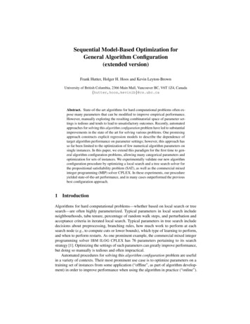
new , θinc , M, R, tintensif y , Π, ĉ)Procedure 2: Intensify(Θĉ(θ, Π 0 ) denotes the empirical cost of θ on the subset of instances Π 0 Π, based on theruns in R; maxR is a parameter, set to 2 000 in all our experiments new ; incumbent parameter setting,Input : Sequence of parameter settings to evaluate, Θθinc ; model, M; sequence of target algorithm runs, R; time bound, tintensif y ;instance set, Π; cost metric, ĉOutput : Updated sequence of target algorithm runs, R; incumbent parameter setting, θinc new ) do1 for i : 1, . . . , length(Θ new [i];2θnew Θ3if R contains less than maxR runs with configuration θinc then4Π 0 {π 0 Π R contains less than or equal number of runs using θinc and π 0than using θinc and any other π 00 Π} ;5π instance sampled uniformly at random from Π 0 ;6s seed, drawn uniformly at random;7R ExecuteRun(R, θinc , π, s);89101112131415161718193.1N 1;while true doSmissing hinstance, seedi pairs for which θinc was run before, but not θnew ;Storun random subset of Smissing of size min(N, Smissing );foreach (π, s) Storun do R ExecuteRun(R, θnew , π, s);Smissing Smissing \ Storun ;Πcommon instances for which we previously ran both θinc and θnew ;if ĉ(θnew , Πcommon ) ĉ(θinc , Πcommon ) then break;else if Smissing then θinc θnew ; break;else N 2 · N ;if time spent in this call to this procedure exceeds tintensif y and i 2 then break;return [R, θinc ];Generalization I: An Intensification Mechanism for Multiple InstancesA crucial component of any algorithm configuration procedure is the so-called intensification mechanism, which governs how many evaluations to perform with eachconfiguration, and when to trust a configuration enough to make it the new current bestknown configuration (the incumbent). When configuring algorithms for sets of instances,we also need to decide which instance to use in each run. To address this problem,we generalize TB-SPO’s intensification mechanism. Our new procedure implements avariance reduction mechanism, reflecting the insight that when we compare the empiricalcost statistics of two parameter configurations across multiple instances, the variance inthis comparison is lower if we use the same N instances to compute both estimates.Procedure 2 defines this new intensification mechanism more precisely. It takes as new , and compares them in turn to the currentinput a list of promising configurations, Θincumbent configuration until a time budget for this comparison stage is reached.11 new , one more configurationIf that budget is already reached after the first configuration in Θis used; see the last paragraph of Section 4.3 for an explanation why.

In each comparison of a new configuration, θnew , to the incumbent, θinc , we firstperform an additional run for the incumbent, using a randomly selected hinstance, seedicombination. Then, we iteratively perform runs with θnew (using a doubling scheme)until either θnew ’s empirical performance is worse than that of θinc (in which casewe reject θnew ) or we performed as many runs for θnew as for θinc and it is still atleast as good as θinc (in which case we change the incumbent to θnew ). The hinstance,seedi combinations for θnew are sampled uniformly at random from those on whichthe incumbent has already run. However, every comparison in Procedure 2 is basedon a different randomly selected subset of instances and seeds, while F OCUSED ILS’sProcedure “better” uses a fixed ordering to which it can be very sensitive.3.2Defining ROARWe now define Random Online Aggressive Racing (ROAR), a simple model-free instantiation of the general SMBO framework (see Algorithm Framework 1).2 This surprisinglyeffective method selects parameter configurations uniformly at random and iterativelycompares them against the current incumbent using our new intensification mechanism.We consider ROAR to be a racing algorithm, because it runs each candidate configurationonly as long as necessary to establish whether it is competitive. It gets its name becausethe set of candidates is selected at random, each candidate is accepted or rejected online,and we make this online decision aggressively, before enough data has been gatheredto support a statistically significant conclusion. More formally, as an instantiation ofthe SMBO framework, ROAR is completely specified by the four components Initialize, FitModel, SelectConfigurations, and Intensify. Initialize performs a single run withthe target algorithm’s default parameter configuration (or a random configuration ifno default is available) on an instance selected uniformly at random. Since ROAR ismodel-free, its FitModel procedure simply returns a constant model which is never used.SelectConfigurations returns a single configuration sampled uniformly at random fromthe parameter space, and Intensify is as described in Procedure 2.4Sequential Model-based Algorithm Configuration (SMAC)In this section, we introduce our second, more sophisticated instantiation of the generalSMBO framework: Sequential Model-based Algorithm Configuration (SMAC). SMACcan be understood as an extension of ROAR that selects configurations based on a modelrather than uniformly at random. It instantiates Initialize and Intensify in the same wayas ROAR. Here, we discuss the new model class we use in SMAC to support categoricalparameters and multiple instances (Sections 4.1 and 4.2, respectively); then, we describehow SMAC uses its models to select promising parameter configurations (Section 4.3).Finally, we prove a convergence result for ROAR and SMAC (Section 4.4).2We previously considered random sampling approaches based on less powerful intensificationmechanisms; see, e.g., R ANDOM defined in [19].

4.1Generalization II: Models for Categorical ParametersThe models in all existing SMBO methods of which we are aware are limited to numericalparameters. In this section, in order to handle categorical parameters, we adapt themost prominent previously used model class (Gaussian stochastic process models) andintroduce the model class of random forests to SMBO.A Weighted Hamming Distance Kernel Function for GP Models. Most recent workon sequential model-based optimization [15, 16, 18] uses Gaussian stochastic processmodels (GPs; see [20]). GP models rely on a parameterized kernel function k : Θ Θ 7 R that specifies the similarity between two parameter configurations. Previous SMBOapproaches for numerical parameters typically choose the GP kernel function" d#X2k(θi , θj ) exp( λl · (θi,l θj,l ) ) ,(1)l 1where λ1 , . . . , λd are the kernel parameters.For categorical parameters, we define a new, similar kernel. Instead of measuring the(weighted) squared distance, it computes a (weighted) Hamming distance:#" dXkcat (θi , θj ) exp( λl · [1 δ(θi,l , θj,l )]) ,(2)l 1where δ is the Kronecker delta function (ones if its two arguments are identical and zerootherwise).For a combination of continuous parameters Pcont and categorical parameters Pcat ,we apply the combined kernel"#XX2Kmixed (θi , θj ) exp( λl · (θi,l θj,l ) ) ( λl · [1 δ(θi,l , θj,l )]) .l Pcontl PcatAlthough Kmixed is a straightforward generalization of the standard Gaussian kernel inEquation 1, we are not aware of any prior use of this kernel or proof that it is indeed avalid kernel function.3 We provide this proof in the appendix. Since Gaussian stochasticprocesses are kernel-based learning methods and since Kmixed is a valid kernel function,it can be swapped in for the Gaussian kernel without changing any other componentof the GP model. Here, we use the same projected process (PP) approximation of GPmodels [20] as in TB-SPO [19].Random Forests. The new default model we use in SMAC is based on random forests[24], a standard machine learning tool for regression and classification. Random forestsare collections of regression trees, which are similar to decision trees but have real3Couto [23] gives a recursive kernel function for categorical data that is related since it is alsobased on a Hamming distance.

values (here: target algorithm performance values) rather than class labels at their leaves.Regression trees are known to perform well for categorical input data; indeed, theyhave already been used for modeling the performance (both in terms of runtime andsolution quality) of heuristic algorithms (e.g., [25, 26]). Random forests share this benefitand typically yield more accurate predictions [24]; they also allow us to quantify ouruncertainty in a given prediction. We construct a random forest as a set of B regressiontrees, each of which is built on n data points randomly sampled with repetitions fromthe entire training data set {(θ1 , o1 ), . . . , (θn , on )}. At each split point of each tree, arandom subset of dd · pe of the d algorithm parameters is considered eligible to be splitupon; the split ratio p is a parameter, which we left at its default of p 5/6. A furtherparameter is nmin , the minimal number of data points required to be in a node if it isto be split further; we use the standard value nmin 10. Finally, we set the number oftrees to B 10 to keep the computational overhead small.4 We compute the randomforest’s predictive mean µθ and variance σθ2 for a new configuration θ as the empiricalmean and variance of its individual trees’ predictions for θ. Usually, the tree predictionfor a parameter configuration θn 1 is the mean of the data points in the leaf one ends upin when propagating θn 1 down the tree. We adapted this mechanism to instead predictthe user-defined cost metric of that data, e.g., the median of the data points in that leaf.Transformations of the Cost Metric. Model fit can often be improved by transformingthe cost metric. In this paper, we focus on minimizing algorithm runtime. Previous workon predicting algorithm runtime has found that logarithmic transformations substantiallyimprove model quality [27] and we thus use log-transformed runtime data throughout thispaper; that is, for runtime ri , we use oi ln(ri ). (SMAC can also be applied to optimizeother cost metrics, such as the solution quality an algorithm obtains in a fixed runtime;other transformations may prove more efficient for other metrics.) However, we notethat in some models such transformations implicitly change the cost metric users aim tooptimize. For example, take a simple case where there is only one parameter configuration θ for which we measured runtimes (r1 , . . . , r10 ) (21 , 22 , . . . , 210 ). While the truearithmetic mean of these runs is roughly 205, a GP model trained on this data using a logtransformation would predict the mean to be exp (mean((log(r1 ), . . . , log(r10 )))) 45.This is because the arithmetic mean of the logs is the log of the geometric mean:v"!#(1/n)u nnXuYngeometric mean txi explog(xi )i 1" expi 1n#1Xlog(xi ) exp (mean of logs).n i 1For GPs, it is not clear how to fix this problem. We avoid this problem in our randomforests by computing the prediction in the leaf of a tree by “untransforming” the data,computing the user-defined cost metric, and then transforming the result again.4An optimization of these three parameters might improve performance further. We plan onstudying this in the context of an application of SMAC to optimizing its own parameters.

4.2Generalization III: Models for Sets of Problem InstancesThere are several possible ways to extend SMBO’s models to handle multiple instances.Most simply, one could use a fixed set of N instances for every evaluation of the targetalgorithm run, reporting aggregate performance. However, there is no good fixed choicefor N : small N leads to poor generalization to test data, while large N leads to aprohibitive N -fold slowdown in the cost of each evaluation. (This is the same problemfaced by the PARAM ILS instantiation BASIC ILS(N) [8].) Instead, we explicitly integrateinformation about the instances into our response surface models. Given a vector offeatures xi describing each training problem instance πi Π, we learn a joint model thatpredicts algorithm runtime for combinations of parameter configurations and instancefeatures. We then aggregate these predictions across instances.Instance Features. Existing work on empirical hardness models [28] has demonstratedthat it is possible to predict algorithm runtime based on features of a given probleminstance. Most notably, such predictions have been exploited to construct portfolio-basedalgorithm selection mechanisms, such as SATzilla [29, 27].For SAT instances in the form of CNF formulae, we used 126 features includingfeatures based on graph representations of the instance, an LP relaxation, DPLL probing,local search probing, clause learning, and survey propagation. All features are listed inFigure 2. For MIP instances we computed 39 features, including features based on graphrepresentations, an LP relaxation, the objective function, and the linear constraint matrix.All features are listed in Figure 3. To reduce the computational complexity of learning,we applied principal component analysis (see, e.g., [30]), to project the feature matrixinto a lower-dimensional subspace spanned by the seven orthogonal vectors along whichit has maximal variance.For new domains, for which no features have yet been defined, SMAC can stillbe applied with an empty feature set or simple domain-independent features, such asinstance size or the performance of the algorithm’s default setting (which, based onpreliminary experiments, seems to be a surprisingly effective feature). Note that incontrast to per-instance approaches, such as SATzilla [29, 27], instance features areonly needed for the training instances: the end result of algorithm configuration is asingle parameter configuration that is used without a need to compute features for testinstances. As a corollary, the time required for feature computation is not as crucial inalgorithm configuration as it is in per-instance approaches: in per-instance approaches,feature computation has to be counted as part of the time required to solve test instances,while in algorithm configuration no features are computed for test instances at all. Infact, features for the training instances may well be the result of an extensive offlineanalysis of those training instances, or can even be taken from the literature. Computingthe features we used here took an average of 30 seconds for the SAT domains, and 4.4seconds for the

programming solver IBM ILOG CPLEX has 76 parameters pertaining to its search strategy [1]. Optimizing the settings of such parameters can greatly improve performance, but doing so manually is tedious and often impractical. Automated procedures for solving this algorithm configuration problem are useful in a variety of contexts.