WIXLIB

*Fig. 4. Traffic networkpd ,1, Rtd ,1,offpd ,1,Gpc ,1αtc ,0 01pd ,2, Rtd ,1,ontd ,2,offpc ,2α10 α11tc ,1pd ,2,Gpc ,3α 20 α 21tc ,2td ,2,onpc ,4α 30 α 31tc ,3pc ,5α 40 α 41tc ,4α 50tc ,5Fig. 5. Hybrid Petri Net model of traffic networkt2 respectively, a and b are the arc weights given by the incidence relationship. The behavioris illustrated in Fig.2 and Fig.3.Figure 5 shows the HPN model for the road of Fig.4. In Fig.5, each section i of li -meterslong constitutes the straight road, and two traffic lights are installed at the point of crosswalk.pc Pc represents each section of the road, and has maximum capacity (maximum numberof vehicles). Also, pd Pd represents the traffic signal where green signal is indicated by anexistence of a token. Note that each signal is supposed to have only two states ‘go (green)’ or‘stop (red)’ for simplicity.T is the set of continuous transitions which represent the boundaryof two successive sections. q j (τ ) is the firing speeds assigned to transition t j T at time τ.q j (τ ) represents the number of vehicles passing through the boundary per time unit of twosuccessive sections(measuring position) at time τ. The sensors to capture the number of thevehicles are supposed to be installed at every boundary of the section as show in Fig.4. Theelement of I ( p, t) is always 0 or αij . αij is the number of traffic lanes in each section. Finally, M0is specified as the initial marking of the place p P. The net dynamics of HPN is representedby a simple first order differential equation for each continuous place pci Pc as follows:if pd,k t j is not null,dmC,i (τ ) I ( pci , t j ) · q j (τ ) · mD,k (τ ),dtt j p ci p ci(3)dmC,i (τ ) I ( p ci , t j ) · q j ( τ ),dtt j p ci p ci(4)otherwise,where mC,i (τ ) is the marking for the place pci ( Pc ) at time τ, and m D,k (τ ) is the marking forthe place pdk ( Pd ). The equation (3) is transformed to its discrete-time version supposingwww.intechopen.com

# %&& that q j (τ ) is constant during two successive sampling instants as follows:mC,i ((κ 1) Ts ) mC,i (κTs ) t j p ci p ciI ( pci , t j ) · q j (κTs ) · m D,j (κTs ) · Ts .(5)where κ is sampling index, and Ts is sampling period.Note that the transition t is enabled at the sampling instant κTs if the marking of its preceding discrete place pd j Pd satisfies m D,j (κ ) I ( pd j , t). Also if t does not have any input(discrete) place, t is always enabled.2.2 Definition of flow qiIn order to derive the flow behavior, the relationship among qi (τ ), k i (τ ) and vi (τ ) must bespecified. One of the simple ideas is to use the well-known modelqi ( τ )(k i (τ ) k i 1 (τ )) vi (τ ) vi 1 (τ )22 (6)supposing that the density k i (τ ) and k i 1 (τ ), and average velocity vi (τ ) and vi 1 (τ ) of theflow in i and (i 1)th sections are almost identical. Then, by incorporating the velocity model ki (τ ),(7)vi ( τ ) v f i · 1 k jamwith (6), the flow dynamics can be uniquely defined. Here, k jam is the density in which thevehicles on the roadway are spaced at minimum intervals (traffic-jammed), and v f i is themaximum speed, that is, the velocity of the vehicle when no other vehicle exists in the samesection.If there exists no abrupt change in the density on the road, this model is expected to workwell. However, in the urban traffic network, this is not the case due to the existence of theintersections controlled by the traffic signals. In order to treat the discontinuities of the densityamong neighboring sections (i.e. neighboring continuous places), the idea of ‘shock wave’(10)is introduced as follows. We consider the case as shown in Fig.6 where the traffic density ofith section is lower than that of (i 1)th section in which the boundary of density differencedesignated by the dotted line is moving forward. Here, the movement of this boundary iscalled shock wave and the moving velocity of the shock wave ci (τ ) depends on the densitiesand average velocities of ith and (i 1)th sections as follows:ci ( τ ) v i ( τ ) k i ( τ ) v i 1 ( τ ) k i 1 ( τ ).k i ( τ ) k i 1 ( τ )(8)The traffic situation can be categorized into the following four types taking into account thedensity and shock wave.(C1) k i (τ ) k i 1 (τ ), and ci (τ ) 0,(C2) k i (τ ) k i 1 (τ ), and ci (τ ) 0,(C3) k i (τ ) k i 1 (τ ),www.intechopen.com

NYL YLNL NLQPGL WK GLVWULFW2EVHUYLQJ SRVLWLRQNL WK GLVWULFW0RYHPHQW RI VKRFN ZDYHFLYL YLNL NLQPGL WK GLVWULFW2EVHUYLQJ SRVLWLRQL WK GLVWULFWFig. 6. Movement of shock wave in the case of k i (τ ) k i 1 (τ ) and ci (τ ) 0(C4) k i (τ ) k i 1 (τ ) (no shock wave).Firstly, in both cases of (C1) and (C2) where k i (τ ) is smaller than k i 1 (τ ), the vehicles passingthrough the density boundary (dotted line) reduce their speeds. The movement of the shockwave is illustrated in Fig.6 (ci (τ ) 0) and Fig.7 (ci (τ ) 0). In Fig.6 and Fig.7, the ‘measuring position’ implies the position where transition ti is assigned. Since the traffic flow qi (τ )represents the numbers of vehicles passing through the measuring position per unit time, inthe case of (C1), it can be represented by n m in Fig.6, where n and m represent the area ofthe corresponding rectangular, i.e. the product of the vi (τ ) and k i (τ ). Similarly, in the case of(C2), qi (τ ) can be represented by m in Fig.7.These considerations lead to the following models:in the case of (C1)www.intechopen.com

,# qi ( τ ) vi ( τ ) k i ( τ ) ki (τ )k i ( τ ),v fi 1 k jam %&& (9)(10)in the case of (C2)qi ( τ ) v i 1 ( τ ) k i 1 ( τ )(11) k (τ )k i 1 ( τ ).(12) v f i 1 1 i 1k jamIn the cases of (C3) and (C4) where k i (τ ) is greater than k i 1 (τ ), the vehicles passing throughthe density boundary come to accelerate. In this case, the flow can be well approximatedby taking into account the average density of neighboring two sections. This is intuitivelybecause the difference of the traffic density is going down. Then in the cases of (C3) and (C4),the traffic flow can be formulated as follows:in the cases of (C3) and (C4),qi ( τ ) k i ( τ ) k i 1 ( τ )2 v f (τ ) 1 k i ( τ ) k i 1 ( τ )2k jam .(13)As the results, the flow model (9) (13) taking into account the discontinuity of the densitycan be summarized as follows: k (τ ) k (τ ) k i (τ ) k i 1 (τ )ii 1v1 f 22k jam i f k i ( τ ) k i 1 ( τ ) k (τ )ki (τ )v f i 1 kijamqi ( τ ) .(14) ifk(τ) k ii 1 ( τ ) and c ( τ ) 0 k (τ ) k i 1 ( τ )v f i 1 1 i k 1 jam i f k i (τ ) k i 1 (τ ) and c(τ ) 0Figure 8 shows the HPN model of the ith intersection, where the notation for other than southwardly entrance lane is omitted. In Fig.8, l j,E , l j,W , l j,S and l j,N are the length of the corresponding districts, and the numbers of the vehicles in the districts are obtained as for examplepc,jIS (τ ) k jIS (τ ) · l j,S . The vehicles in pc,jIS are assumed to have the probability ζ j,SW , ζ j,SN ,and ζ j,SE to proceed into the district corresponding to pc,jOW , pc,jON , and pc,jOE as follows,www.intechopen.comk jSW (τ ) k jIS (τ )ζ j,SW (τ ),(15)k jSN (τ ) k jIS (τ )ζ j,SN (τ ),(16)k jSE (τ ) k jIS (τ )ζ j,SE (τ ).(17)

-NYL YLNL NLQPGL WK GLVWULFW2EVHUYLQJ SRVLWLRQ0RYHPHQW RI VKRFN ZDYHFLL WK GLVWULFWNYL YLNL NLQPGL WK GLVWULFW2EVHUYLQJ SRVLWLRQL WK GLVWULFWFig. 7. Movement of shock wave in the case of k i (τ ) k i 1 (τ ) and ci (τ ) 0Note that these probabilities are determined by the traffic network structure, and satisfy at τ,0 ζ j,SW (τ ) 1,0 ζ j,SN (τ ) 1,0 ζ j,SE (τ ) 1,ζ j,SW (τ ) ζ j,SN (τ ) ζ j,SE (τ ) 1.Therefore, the traffic flows of the three directions are represented with q k jSN (τ ), k jON (τ ) ,q k jSW (τ ), k jOW (τ ) ,q k jSE (τ ), k jOS (τ ) .(18)(19)(20)(21)(22)(23)(24)Note that the mutual exclusion of the same traffic light with the intersecting road is represented in the Fig.8.www.intechopen.com

# %&& l j,Nl j ,Wpc , jONl j,Ek jONpc , jOEtd , j ,offk jOEpd , j ,Gpd , j , Rpc , jOWtd , j ,onk jOWNl j ,SWpc , jISEk jISSFig. 8. Hybrid Petri Net model of intersection2.3 Derived flow modelIn this subsection, we confirm the effectiveness of the proposed traffic flow model developedin the previous subsection by comparing it with the microscopic model. The usefulness ofCellular Automaton (CA) in representing the traffic flow behavior was investigated in (3).Some of well-known traffic flow simulators such as TRANSIMS and MICROSIM are based onCA model.The essential property of CA is characterized by its lattice structure where each cell representsa small section on the road. Each cell may include one vehicle or not. The evolution of CA isdescribed by some rules which describe the evolution of the state of each cell depending onthe states of its adjacent cells.The evolution of the state of each cell in CA model can be expressed byoutn j (τ 1) ninj ( τ )(1 n j ( τ )) n j ( τ ),(25)where n j (τ ) is the state of cell j which represents the occupation by the vehicle (n j (τ ) 0implies that the jth cell is empty, and n j (τ ) 1 implies that a vehicle is present in the jthcell at τ). ninj ( τ ) represents the state of the cell from which the vehicle moves to the jth cell,and noutj ( τ ) indicates the state of the destination cell leaving from the jth cell. In order to findoutninj ( τ ) and n j ( τ ), some rules are adopted as follows:Step 1, Acceleration rule: All vehicles, that have not reached at the speed of maximum speedv f , accelerate its speed v j (τ ) by one unit velocity vunit as follows:v j (τ Δτ ) v j (τ ) vunit .www.intechopen.com(26)

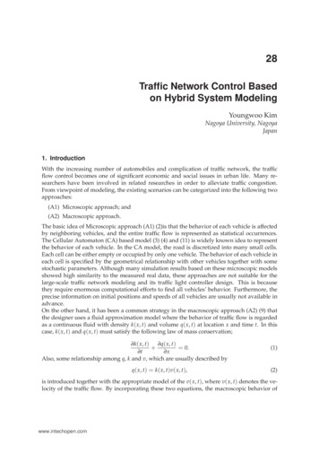
Step 2, Safety distance rule: If a vehicle has e empty cells in front of it, then the velocity at thenext time instant v j (τ Δτ ) is restricted as follows:v j (τ Δτ ) min{e, v j (τ Δτ )}.(27)Step 3, Randomization rule: With probability p, the velocity is reduced by one unit velocityas follows:v j (τ Δτ ) v j (τ Δτ ) p · vunit .(28)Figure 9 shows the behavior of traffic flow obtained by applying the CA model to the two successive sections which is 450[m] long. The parameters used in the simulation are as follows:computational interval Δτ is 1 [sec], each cell in the CA is assigned to 4.5 [m]-long interval onthe road, maximum speed v f is 5 (cells/Δτ), which is equivalent to 81 [Km/h] ( 4.5[m/cell] ·5 [cells/Δτ] · 3600[sec]/1000). The left figure of Fig.9 shows the obtained relationship amongnormalized flow qi (τ ) and densities k i (τ ) and k i 1 (τ ). The right small figure is the abstractedillustration of the real behavior.First of all, we look at the behavior along the edge a in the right figure which implies the casethat the traffic signal is changed from red to green. At the point of k i (τ ) 0 and k i 1 (τ ) 0,the traffic flow qi (τ ) becomes zero since there is no vehicle in both ith and (i 1)th section.Then, qi (τ ) is proportionally increased as k i (τ ) increases, and reaches the saturation point(k i (τ ) 0.9). Next, we look at the behavior along the edge b which implies that the ith sectionis fully occupied. In this case, the maximum flow is measured until the density of the (i 1)thsection is reduced by 50% (i.e. k i 1 (τ ) 0.5), and after that the flow goes down according tothe increase of k i 1 (τ ). Although CA model consists of quite simple procedures, it can showquite natural traffic flow behavior.On the other hand, Fig.10 shows the behavior in case of using HPN where the proposed flowmodel given by (14) is embedded. We can see that Fig.10 shows the similar characteristics toFig.9, especially, the saturation characteristic is well represented despite of the use of macroscopic model. As another simple modeling strategy, we consider the case that the average oftwo k i (τ ) and k i 1 (τ ) are used to decide the flow qi (τ ) (i.e. use (13) ) for all cases. Figure 11shows the behavior in case of using HPN where the flow model is supposed to be given by (13)for all cases. Although the qi (τ ) shows similar characteristics in the region of k i (τ ) k i 1 (τ ),at the point of k i (τ ) 0 and k i 1 (τ ) k jam , qi (τ ) takes its maximum value. This obviouslycontradicts to the natural flow behavior.Before concluding this subsection, it is worthwhile to compare the computational amount. Incase of using CA, it took 140 seconds to construct the traffic flow dynamics using Athlon XP2400 and Windows 2000, while only 0.06 seconds in case of using HPN and (14).3. Model Predictive Control of Traffic Network Control based on MLDS descriptionThe Receding Horizon Control (RHC) or Model Predictive Control (MPC) is one of well known paradigms for optimizing the systems with constraints and uncertainties. In RHCparadigms, the solutions are elements of finite dimensional vector spaces, and finite-horizonoptimization is carried out in order to provide stability or performance analysis. However, theapplication of RHC has been mainly restricted to the system with sufficiently long samplinginterval, since finite-horizon optimization is computationally demanding.This chapter firstly formulate the traffic flow model developed in chapter 2 in the form ofMLDS description coupled with RHC strategy, where wide range of traffic flow is considered.www.intechopen.com

,''# %&& 7UDIILF IORZ TL 7UL DIIL W FGK G HQ LVW VLW\ULF R IWN L NL LVWULFW I L WK G R\WLVLF G H Q7UDII D%E&Fig. 9. Traffic flow behavior obtained from CA modelThis formulation is recast to the canonical form of 0-1 Mixed Integer Linear Programming(MILP) problem to optimize its behavior and a new Branch and Bound (B&B) based algorithmis presented in order to abate computational cost of MILP problem.3.1 MLDS representation of TCCS based on Piece-Wise Affine (PWA) linearization of trafficflowSince TCCS is the hybrid dynamical system including both continuous traffic flow dynamicsand discrete aspects for traffic light signal control, some algebraic formulation, which handlesboth continuous and discrete behaviors, must be introduced. The MLDS description has beendeveloped to describe such class of systems considering some constraints shown in the formof inequalities and can be combined with powerful search engine such as Mixed Integer LinearProgramming (MILP).The MLDS (12) description can be formalized as following.x ( τ 1)y(τ )E2τ δ(τ ) Aτ x(τ ) B1τ u(τ ) B2τ δ(τ ) B3τ z(τ )Cτ x(τ ) D1τ u(τ ) D2τ δ(t) D3τ (τ )E3τ z(τ ) E1τ u(τ ) E4τ x(τ ) E5τ(29)(30)(31)In MLDS formulation, (29), (30) and (31) are state equation, output equation and constraintinequality, respectively, where x, y and u are the state, output and input variable, whose components are constituted by continuous and/or 0-1 binary variables, δ(τ ) {0, 1} and z(τ ) ℜwww.intechopen.com

,'(Fig. 10. Traffic flow behavior obtained from the proposed traffic flow modelrepresent auxiliary logical and continuous variables. By introducing the constraint inequality of (31), non-linear constraints as (14) can be transformed to the computationally tractablePiece-Wise Affine (PWA) forms.The traffic flow of Fig. 9 can be approximated as the right figure of Fig. 9 which consists ofthree planes as follows,Plane A: The traffic flow qi is saturated (k i (τ ) a and k i 1 (τ ) (k jam a))Plane B: The traffic flow qi is mainly affected by the quantity of traffic density k i (τ ) (k i (τ ) a and k i (τ ) k i 1 k jam )Plane C: The traffic flow qi is mainly affected by the quantity of traffic density k i 1 (τ )(k i 1 (τ ) k jam a and k i (τ ) k i 1 k jam )where a is the threshold value to describe saturation characteristic of traffic flow that if k i (τ ) a and/or k i 1 (τ ) k jam a, the value of qi (τ ) hovers at its maximum value qmax .www.intechopen.com

,')# %&& 7UDIILF IORZ TL L DIIL W F G K G HQLVW VLW\ ULF RI W 7UNL FW N LL GLVWUW RI L K \WLVHQILF G7UDIFig. 11. Traffic flow behavior obtained by averaging k i and k i 1Fig.12 shows three planes partitioned by introducing three auxiliary variables δP,i,1 (τ ),δP,i,2 (τ ) and δP,i,3 (τ ) which are defined as follows,[δP,i,1 (τ ) 1] ki (τ ) k i 1 ( τ ) ak jam a[δP,i,2 (τ ) 1] ki (τ ) k i ( τ ) k i 1 ( τ )[δP,i,3 (τ ) 1] k i 1 ( τ ) k i ( τ ) k i 1 ( τ )(32) a εk jam(33) k jam a εk jam ε(34)δP,i,1 (τ ) δP,i,2 (τ ) δP,i,3 (τ ) 1(35)where ε is small tolerance to consider equality sign.Therefore, the traffic flow qi (τ ) can be rewritten in a compact form as followsqi ( τ ) qmax k i (τ )δP,i,2 (τ )aqmax (1 k i 1 (τ )) δP,i,3 (τ )aqmax δP,i,1 (τ ) 3 i 1www.intechopen.comδP,i,j (τ ) 1(36)

,'*Fig. 12. Assignation of planes by introducing auxiliary variableswhere 0 k i (τ ) k jam , 0 k i 1 k jam ( 1), qmax is the maximum value of traffic flow.Figure xxx shows the piece-wise affine (PWA) dynamics of the traffic flow model developedin the previous chapter where a 0.3 and qmax 1.The equations (32) to (34) can be generalized as (37) and (38), and transformed to inequalityas (39) The equations (32) and (34) can be generalized as (37) and (38), and transformed toinequality as (39)[δP,i,j (τ ) 1] j kik i 1 kik i 1 j: S j ki (τ ) Tj(37) (38)where ki (τ) [k i (τ )k i 1 (τ )] T and S j and Tj are the matrices with suitable dimensions whichsatisfyS j ki ( τ ) Mj Tj Mj [1 δP,i,j (τ )],(39)max S j ki (τ ) Tj .ki j(40)The traffic flow qi (τ ) of (37) is the relationship between ki (τ) and δP,i (τ) [δP,i,1 (τ ) δP,i,2 (τ ) δP,i,3 (τ )] which can be rewritten as follows,qi ( τ ) f (δP,i (τ ), ki 1 (τ ))3 j ( Fi (τ )ki (τ ) Hi )δP,i,j (τ )j 1www.intechopen.comj(41)(42)

,' # j′ %&& jwhere δP,i [δP,i,1 , δP,i,2 , δP,i,3 ] . In these equations, each pair of Fi and Hi represents thecorresponding domain of Fig. 12 as follows,Fi1 [ 0Hi1Fi2Hi2Fi3 qmaxHi3 0 ](43)(44)qmaxa [ 0(46) ][ 0 qmaxaqmaxa(47)0 ](45)(48)The traffic flow zi (τ) [zi,1 (τ ) zi,2 (τ ) zi,3 (τ )] in consideration of the binary input ui (τ ) {0, 1} for traffic light control can be represented byzi,j (τ )zi,j (τ )zi,j (τ ) Mi ui (τ )δP,i,j (τ ),(49)mi ui (τ )δP,i,j (τ ),(50) jFi ki (τ ) jHi mi (1 ui (τ )δP,i,j (τ )),zi,j (τ )jFi ki (τ ) (51)jHi Mi (1 ui (τ )δP,i,j (τ )).(52)where Mi and mi are respectivelyMimi jFi ki (τ ) H j ,(53)Fi ki (τ ) H j .minki (τ ) j(54)maxki (τ ) j jThe product ui (τ ) δP,i,j (τ ) can be replaced by an auxiliary logical variable δM,i,j (τ ) ui (τ )δP,i,j (τ ) in order to make it tractable to deal with MILP problem. Then this relationship can beequivalently represented as follows, ui (τ ) δM,i,j (τ ) δP,i,j (τ ) δM,i,j (τ )ui (τ ) δP,i,j (τ ) δM,i,j (τ ) 0,(55)0,(56)1.(57)Therefore, the MLDS description for the proposed system can be formalized as follows,x (κ 1)z (κ )E2 δ (κ ) Ax(κ ) Bz(κ ),(58)C1 diag(u(κ ))C2 δ(κ ),(59)E3 z (κ )E1 u (κ ) E4 x (κ ) E5(60)where the element xi (κ ) of x(κ ) ℜ P , is marking of the place pci at the sampling instance κ,the element ui (κ )( {

0 Traf c Network Control Based on Hybrid System Modeling Youngwoo Kim Nagoya University, Nagoya Japan 1. Introduction With the increasing number of automobiles and complication of traf c network, the traf c