Transcription
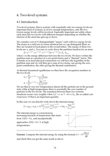
4. Two-level systems4.1 IntroductionTwo-level systems, that is systems with essentially only two energy levels areimportant kind of systems, as at low enough temperatures, only the twolowest energy levels will be involved. Especially important are solids whereeach atom has two levels with different energies depending on whether theelectron of the atom has spin up or down.We consider a set of N distinguishable ”atoms” each with two energy levels.The atoms in a solid are of course identical but we can distinguish them, asthey are located in fixed places in the crystal lattice. The energy of these twolevels are ε0 and ε1 . It is easy to write down the partition function for an atomZ e ε0 / kB T e ε1 / kBT e ε 0 / k BT (1 e ε / kB T ) Z0 Ztermwhere ε is the energy difference between the two levels. We have written thepartition sum as a product of a zero-point factor and a “thermal” factor. Thisis handy as in most physical connections we will have the logarithm of thepartition sum and we will then get a sum of two terms: one giving the zeropoint contribution, the other giving the thermal contribution.At thermal dynamical equilibrium we then have the occupation numbers inthe two levelsNNn0 e ε 0 / kBT Z1 e ε / k BTNNe ε /k BTn1 e ε 1 /k BT Z1 e ε /k BTWe see that at very low temperatures almost all the particles are in the groundstate while at high temperatures there is essentially the same number ofparticles in the two levels. The transition between these two extremesituations occurs very roughly when kBT ε or T θ ε /kB , the so-called scaletemperature θ that is an important quantity.In this case we can directly write down the internal energyε e ε0 /kBT ε1e ε1 /kBTN ε e θ /TE n0ε 0 n1ε1 N 0 ε0 /kBT Nε 01 e θ /Te e ε1 /kBTThe internal energy is a monotonousincreasing function of temperature that startsfrom E ( 0 ) N ε 0 and asymptoticallyapproaches E ( 0 ) N ε / 2 at –––––– ln ZExercise. Compute the internal energy by using the formula E N βand check that you get the same result as above.31
�When we now know the internal energy as a function of temperature we caneasily compute the heat capacity of the system as a function of �––––Exercise: Use the graph above to make a sketch of how the heat capacitydepends on �––––We haveθ /T ) e θ /T(dEc NkB2dT1 e θ /T2()The result is somewhat unexpected. The heat capacity has a maximum oforder Nk B at a temperature that is approximately the scale temperature (moreprecisely for T 0.417 θ ). At low temperatures the heat capacity approaches 2 θ /Tzero quit fast, like T e. At high temperatures the heat capacity also goes 2to zero like T . This behaviour is typical for atwo-level system and is called a Schottkyanomaly. That the heat capacity goes to zero asthe temperature goes to zero is universal forany system. As we have seen this is requiredunless the entropy becomes singular (infinite).We can understand the heat capacity curve byqualitative reasoning. At low temperatures the distance between the energylevels is so large that it is very difficult to excite thermally the particles fromthe ground state, this implies a small heat capacity. As the temperature thenapproaches the scale temperature it is easy to excite the particles and you geta large heat capacity. At higher temperatures we have essentially the samenumber of particles in the levels and that situation does not change verymuch as we increase the temperature. This means that the system does notincrease very much its internal energy when the temperature increases: theheat capacity will be small again.We could now compute the entropy fromS NkB ln Z E/Tbut instead we will use another method that further on will be quite useful.Suppose that we study the internal energy E E (S,V , N ) . For the differentialwe havedE TdS pdV µdNThe internal energy is a function of the entropy, a quantity that is difficult tomeasure. We would like to change the functional dependence to for instancetemperature T. We writedE TdS SdT SdT pdV µdN d(TS) SdT pdV µdNMove the TS-term to the left side32
d(E TS) SdT pdV µdNIntroduce a new function of state for energy, F E TS , for which weevidently havedF SdT pdV µdNsomething that tells us that F F(T ,V ,N ) , all variables are now easilymeasurable quantities. The function F is called Helmholtz' free energy.But we have also F F FdF dT dV dN T V NIf we identify terms we get F F F S p µ T V NWe can now rewriteS NkB ln Z E/T F E TS NkBT ln ZInserting the expression for Z we getF Nε0 Nk BT ln 1 e θ /Tthat after derivation with respect to temperature gives θ /T )e θ /T ( F θ /T S Nk B ln 1 e T1 e θ /T ()()The entropy goes to zero for small temperatures, as it should, at absolute zerothe system has no degrees of freedom (only one possible microstate). At hightemperatures the entropy approaches the S Nk B ln 2 something that is easyto see is –––Exercise. Why is this limit –––33
*4.2. InterludeIn chemistry we are often interested in having a function of state for theenergy that depends on pressure instead of volume. In chemical reactions thepressure is normally constant. This is easily fixed:dF SdT pdV µdN SdT pdV Vdp Vdp µdN SdT d ( pV) Vdp µdNThis givesdG d( F pV) SdT Vdp µdNwith a new function of stateG G (T, p, N ) F pV E TS pV , Gibb’s energy. For this functionwe have the partial derivatives G G G S V µ T p NAnother function of state that is used in chemistry is the enthalpy, H. We startfromdE TdS pdV µdN TdS pdV Vdp Vdp µdN TdS d(pV ) Vdp µdNThis impliesdH d ( E pV ) TdS Vdp µdNwith H H H T V µ S p NH H (S, p, N )These transformations to get a suitable function of state are called canonicaltransformations.4.3. Magnetic solidsThe electron has spin 1/2 that gives it a magnetic moment z-component µ .The electron behaves as a small magnet. You can also have a magneticmoment because of the orbital movement of the electron in the atom. Finallyyou can also have a magnetic moment due to a spinning nucleus. The electronspin and the orbital movement result in a magnetic moment of order the Bohrmagnetone!µB 0.93 10 2 3 J/T2mThe magnetic moment of the nucleus is of order the nuclear magnetone!µN 5.05 10 2 7 J/T2M p34
If we put an atom or nucleus that has a magnetic moment in a magnetic fieldin the z direction (or rather define the direction of the magnetic field as the zaxis) one of the two (essentially degenerate) energy levels to be displacedupwards by µB , the other one is displaced downwards by µB . The energydifference between the levels is then 2µB . We use the results from our twolevel model. We want each atom to be essentially independent of the otherssuch that it is not influence by the magnetic moment of its neighbours. Wehave this situation in paramagnetic solids.The scale temperature is θ 2 µB/ kB . We observe the following:1. The thermal properties only depend on the quantity θ /T , or for a givenmagnetic field on the ratio B/T .2. If we insert numerical values and assume that B 1 T , the scaletemperature will be of order a few Kelvins for an electron-spin system and afew milliKelvin for nuclear-spin system. At these low temperatures thethermal properties of the system is almost entirely determined by the twolevel system.4.4 Cooling by adiabatic demagnetisationAn interesting application that exploits the properties of a paramagnetic solidis cooling by adiabatic demagnetisation. We will now describe this process.The paramagnetic solid is put in good thermal contact wit a cooling medium,most often liquid helium. A strong magnetic field is applied. This increasesthe gap between the energy levels and forces the spins to line up in thedirection of the magnetic field that means that the electrons occupy theground state. This in turn means that the paramagnetic solid rids itself ofenergy that is taken up by the cooling medium. We now isolate thermally theparamagnetic solid and then let the magnetic field go to zero. We will thenhave a situation where the major part of the electrons occupy the lowerenergy level, the ground state. As we have now removed the magnetic field,the higher energy level is very close to the ground level but contains very fewelectrons. This corresponds to a very low temperature. We can also interpretwhat is happening by studying how the entropy depends on temperature.The two curves describe precisely the same mathematical function but havedifferent scale temperatures, as they are proportional to the strength of themagnetic field. The path from A to B corresponds to an increase in thestrength of the magnetic field while keeping the temperature constant. Thepath B to C corresponds to an adiabatic decrease (no change in entropy dQ 35
0) of the magnetic field but now with the system isolated from the outsideworld. This means that we change the scale temperature back to what it wasbefore but move along a line parallel to the T axis. The entropy curves areuniversal functions meaning thatSC (θ C /TC ) SB (θB /TB ) θC /TC θ B /TB BC /TC BB /TBorBTC TB CBBThe final temperature depends on how small the magnetic interaction BC isfrom neighbouring atoms. For electron-spin systems you can, using thismethod, reach temperatures as low as 1 mK, for nuclear-spin system the finaltemperature can reach 0.1 µK.4.5. The magnetisationThe magnetisation M is the net sum of all magnetic moment. We havee ε 0 /k BT e ε 1 /k BTM n0 µ n1 ( µ) µN ε 0 / k BT ε 1 / kBT e eµB/ kBT µB/ k BTe eµBµN µB /k BT N µ tanh µB /k BTe ek BTµB, (B large or TkBTsmall) the magnetisation saturates toM Nµ when all magnetic momentshave lined up along the externalµBmagnetic field. For small values ofkBTwe can use a Taylor expansion of thehyperbolic function and getµBM NµkBTIn this approximation themagnetisation is inversely proportionaltemperature. This is Curie’s law thatagrees very well with experiment, seethe diagram.For large values oftoWe can use measurements of the magnetisation as a thermometer! Forelectronic systems we can then measure temperatures down to about 10 mKwhen the magnetic field from internal interactions interfere and also theTaylor expansion requires more terms. Instead we can then use a nuclear-spinsystem and measure somewhat lower temperatures. For really lowtemperatures we can measure the energy split between the energy levelsusing the method of nuclear magnetic resonance (NMR). We then apply aradio frequency to the system with frequency f and use the resonancecondition hf 2µB to select the relevant energy levels. The strength of the36
NMR signal will be proportional to the difference in occupation number ofthe levels, which in turn is proportional 1/T.4.6 Localised one-dimensional harmonic oscillatorsFrom quantum mechanics we have that the energy levels of a harmonicoscillator are given byεn (n 12 )!ω , n 0,1,2 We can now easily write down the partition functionZ e εn / k BT en ( n 12 ) ! ω / kB T e ( n 12 )θ /Tn 12 θ /T e e (n n 12 )θ /T Z0 Ztermnwhere we have introduced the scale temperature θ !ω /k B .In this case we can explicitly sum the partition function, it is a geometricalseries.Z e ( n 12 )θ /Tn e θ /2T e nθ /T n()e θ /2T 1 e θ /T e 2θ /T e θ /2T1 θ /T θ /T1 ee 1The internal energy isE NNk θ ln Z 1N!ω 2 N!ω !ω /kBT 12 NkBθ θ /T B βe 1e 1The first term is the zero-point energy. At hightemperatures the internal energy isE NkBTa result that we derived in an earlier chapter bycounting the number of quadratic terms in the expression for the total energy.However, the quantum mechanical model also gives the behaviour at lowtemperature.θ /T ) eθ /T(dEThe heat capacity is C . NkB2dTeθ /T 12()It starts from zero at T 0 and saturates asexpected for high temperatures at Nk B . Againquantum mechanics describes correctly thebehaviour at low temperatures. We can see theneed for a quantum mechanical description as for low temperatures both theinternal energy and the heat capacity contain Planck’s constant.We can finally compute the entropy from S Fwhere F Nk BT ln Z . ��37
eθ /Tθ /T Exercise. Show that S Nk B ln θ /T θ /T e 1 e 1 Exercise. Show that S 0 when T 0 and S Nk B lnTkT Nk B ln B whenθ!ωT ��Note that also in the high temperature limit the entropy contains Planck’sconstant. Entropy is fundamentally a quantum mechanical quantity. On theother hand the energy and heat capacity can be described classically at hightemperatures.Albert Einstein used the above model with one-dimensional harmonicoscillators in the so-called Einstein model to explain the properties of solids atlow temperatures. The model is qualitatively correct but with closercomparison with experiment it has the wrong temperature dependence.Experiments show that the heat capacity at low temperatures must be3proportional to T . We will in a later chapter present the Debye model that hasa correct T dependence. However, we can already now explain that small heatcapacities of graphite and diamond. As we have seen, the scale temperaturedetermines the transition between the quantum mechanical and classicalregions in temperature, in this case θ !ω /k B . For a harmonic oscillator wehave that the frequency ω k/m where k is the spring constant of the forcebetween the atoms in the solid. Diamond is a very hard solid, thus we canexpect that the spring constants in diamond are very large. This implies thatthe scale temperature is high, about 500 K for diamond. This means that theheat capacity is quite far away from its asymptotic value at room temperatureand that the heat capacity is much below the classical Dulong-Petit value.Even more interesting is the situation with graphite. Themolecular structure of graphite is such that is consists oflayers of carbon atoms with each layer being a very rigidhexagonal lattice. These layers are stacked on top ofeach other and quite loosely connected. This is one of the reasons for graphitebeing used in pencils; the layers are easily ripped off and get attached to thepaper. This is also the reason for graphite being used as a lubricant, thedifferent layers in the graphite can slide relative one another with littlefriction. This structure means that the chemical bindings (the springconstants) are strong in two dimensions, in the hexagonal layer, and weakbetween these layers. We then have two different scale temperatures, a high38
one for vibrations in the layer and a low one for vibrations between the layers.Actually only the vibrations between the layers are activated at roomtemperature. When we count quadratic terms in the total energy we shouldonly count these latter vibrations. This implies that the number of quadraticvibration terms only is 1/3 of the number in a solid where the vibrations canhappen in three dimensions and the heat capacity thus only becomes 1/3 ofthe normal, something that agrees perfectly with experiment.4.7. A note about the partition function for systems withdegenerate energy levelsWe have earlier noted that we should sum over all possible states in thepartition function. This means that if an energy level is degenerate I has to becounted several times, as many times as the degeneracy or the multiplicity ofthe degeneration. Mathematically we write thisZ gi e ε i /k BTiwhere gi is the multiplicity of energy level i. We will use this way of writingvery often when we in the next chapter will treat the statistical description ofgases where we will use so-called group distributions.Exercise problems. Chapter 41. Compute the internal energy of a two-level system using E N ln Zand βcheck that you get the same result as we got in the lecture.2. Assume that we could have a stable equilibrium for a two-level systemwhere we had more particles in the upper level than in the lower one. Whatcan you say about the temperature of such a system? In reality such systemsare not stable but can be realised quasi-stably in for instance a laser bypumping particles to the upper level using external energy. Such systems aresaid to have an inverted population.3. Compute the internal energy and heat capacity for a system with one nondegenerate level with energi 0, two degenerate levels with energy ε and onenondegenerate level with energy 2ε. Hint: Chose a suitable zero-point energy.4. Below what temperature do you have deviations that are larger than 5%from Curie’s law in an ideal electronic spin 1/2 system?5. Magnetisation of Pt nuclei is often used as a thermometer for lowtemperatures. The external magnetic field is 10 mT and the magnetic momentof a Pt nucleus is 0.60 nuclear magnetons. Estimate the usable temperatureinterval of the thermometer if we assume a) that a magnetisation less than1/10 000 of the maximal one cannot be measured with precision and b) thatdeviations from Curie’s law that are larger than 5% are unacceptable.Assume that we use NMR technique to detects the split in the energy levels.What is in this case the NMR frequency?39
6. Experimental results frommeasurements of the specificheat capacity of gadolinium areshown in the figure. At lowtemperatures you see a bump inthe curve caused by a few lowlying energy levels. Explain thisand estimate the distancebetween these levels. Give youranswer in electron volts. Youhave to motivate your answerbut you don’t have to makedetailed computations.Cp[mJ / mol]20001000500200540101520T [K]
5. The ideal gas5.1 Density of statesTo begin with we will consider gases with non-relativistic massive particles.We will need the density of state in energy.We now study bas particles in a “box” with dimensions LxLxL.If we solve the Schödinger equation for such a particle we get wave functionsof the typeϕ ( x, y, z ) Ae ikx x e y e ikz zWe now use so-called periodic boundary conditions where we demand thatϕ x nx L, y n y L, z n y L ϕ ( x, y, z )ik y()This impliesk x nx2π2π2π, ky ny, k z nzLLL2πbetween theLlattice points. Each lattice point corresponds to a state of the gas particle. In anelementary cube we then have exactly one state. The volume of an elementaryIn k-space, these k-values form a cubic lattice with a distance( 2π ) . The density of states in k-space is then 2π cube is evidently L V3( 2π )1/3 V3V( 2π )3You always start with the number of states in an infinitesimal cube in k-spaceand the transform step by step to ε-space:V( 2π )3d3k ( 2π )34π 2 p 2mε V 4π m ( 2m)p dp !3!3( 2π )31/22V( 2π )spherical1 3 symmetryd p !3V3 ε 1/2 dε g ( ε ) dεwhere V is the normalisation volume. The factor 4π comes from that weintegrate over the uninteresting space angles. We have also exploited that themomentum p !k and the relation (in this case) between energy andp2.2mThe relation between energy and momentum/wave vector is called adispersion relation.momentum ε V (2m)This gives the density of states in energy g(ε) 23(2π ) !413 /2ε1/ 2
This expression must be corrected with a spin factor, 2 for spin 1/2 particlesand 3 for (massive) spin 1 particles. The density of states is such thatg ( ε ) dε is the number of states in the energy interval [ ε , ε dε ] .Note 1. It is easy to realise that our box doesn’t have to be cubic. Actually outderivation works for a volume of arbitrary form, thermodynamical propertiesdo not depend on the form of the container.Note 2. We could have used the usual condition when you solve theSchödinger equation in a box, namely that we have standing waves betweenthe walls. This gives a final result that is identical to that we got here but themethod with periodic boundary conditions often is simpler to use.5.2 Group distributionsFirst we observe that the number of states in a gas in a macroscopic volume isenormous and that the energy levels are very close to each other. To handlethis situation we introduce something called group distributions. See the figure!We group such that the number of levels within a group i, gi , is very large,and such that the number of particles within the group, ni , also is large, butsuch that the average distances Δε i between the levels in the different groupsstill is very small. In practice it turns out that you can gi of order 10 and stillhave Δε i 10 9 k B T . It also turns out that it is not critical for the final resulthow we do the grouping.105.3 Identical particlesWe now want to count the number of microstates in a certain distribution. Wethen have to take into account an important fact: particles in a gas arefundamentally identical, that is it is impossible to tell them apart. We cannotdecide which particle occupies a certain state; we can only decide the numberof particles in a certain state. The other important fact is that we have twokinds of particles in nature, fermions and bosons. Fermions follow the Pauliprinciple that says that two fermions cannot be in the same state. Fermionsalways have half integer spin; examples are electrons, protons, and neutrons.Bosons do not follow the Pauli principle; an arbitrary number of bosons can bein the same state. Bosons have integer spin; examples of bosons are photons,helium-4 atoms, and deuterons. This means that we have to count microstates42
differently for fermions and bosons. For fermions we will get Fermi-Dirac(FD) statistics for bosons we will get Bose-Einstein (BE)-statistics.5.4. Counting microstates for fermionsConsider the level group i where we have gi possible states and ni particles tooccupy these states. As we deal with fermions we can have at most oneparticle in each state. Consequently we have gi ni empty states. We then canarrange filled and empty states ingi !ni ! ( gi ni )!ways. The total number of microstates for all levels then isgi !ΩFD i ni ! ( gi ni )!5.5. Counting microstates for bosonsAgain consider level group i. We have gi possible states and ni particles todistribute in these states. We can now have several particles in each statesomething that complicates the counting. However, we can get around thisproblem using a trick. Consider the states as slots with walls in between. Ifthere are gi states there are gi 1 walls between them. Together with the niparticles we now have gi ni 1 objects to handle, gi 1 of one kind (thewalls) and ni of the other kind (the particles) and we can arrange them in( gi ni 1)! ( gi ni )!ni ! ( gi 1)!n i! g i !ways. The total number of microstates for all level is then ΩBE i( gi ni )!ni ! gi !5.6. Dilute gasesNow suppose that we have a dilute gas. By this we mean that ni gi (butstill ni 1 ). This is a very common situation if we for instance consider air atnormal temperature and pressure. In the fermion case we then can make theapproximationg ( g 1) ( gi ni 1) gin igi ! i i ni ! ( gi ni )!ni !ni !In the boson case we have( gi ni )! ( gi ni )( gi ni 1) ( g i 1) g ni ini ! gi !ni !ni !that is we get the same result. This “classical limit” gives us the so-calledMaxwell-Boltzmann (MB) statistics where we havegin iΩ MB ni !i43
5.6. Distributions in thermodynamical equilibrium5.6.1. FermionsWe now copy the procedure that we used for distinguishable particles inchapter 3. We define the entropyS kB ln Ωand try to maximise the entropy given the constraintsN ni and E ε iniiithat is the number of particles and the internal energy are conserved.We maximise the function f gi ln gi ni ln ni ( gi ni ) ln ( gi ni ) α ni N β ε ini E i i iwhere we have used Stirling’s approximation and introduced Lagrangianmultipliers. We compute all partial derivatives with respect to ni and putthem to zero and get after some manipulationgni α βε iie 1It is here useful to define the filling factor, the ratio between the number ofparticles and the number of accessible states in this leveln1fi i α βεigi e 1As the levels are very close we can id we want write this as a continuousdistribution1fFD ( ε ) α βεe 1()5.6.2 BosonsWe repeat the procedure for the boson case and get with a similarcomputation1fBE (ε ) α βεe ��Exercise. Show this by doing the detailed ��––––5.6.3 Dilute gasesFinally, for dilute gases we have1f MB (ε) α βεeExercise. Show ––44
5.7. SummaryAs before β 1/k BT . α can in principle be determined from the condition ni N but it turns out that you can explicitly solve the resulting equationionly in the MB case, we will return to this in the next chapter. If we for theαmoment introduce e B , we can summarize our results in the following way 1 ε / kBT(FD) Be 1 1f (ε ) ε / kBT(MB) Be 0 ε / k1T Be B 1 (BE)As we will see the different kinds of particle system will have very differentphysical properties.45
6. Maxwell-Boltzmann gases6.1. The partition functionWe start by rewriting the filling factor1fi ε i /k BT Ae ε i /k BTBeIn this case we can easily compute A (i.e. implicitly the value of α). We haveN ni gi fi A gi eii ε /k BTiorfi withN ε i /k BTeZZ gi e ε i /k BTithe partition function. This is very similar to what we had before in chapter 3.We now consider a monoatomic gas where the gas atoms have spin zero asfor instance in helium-4. The partition function can be written as an integral asthe energy levels are close3/ 2 ε i / k BTV (2m) 1/ 2 ε / kB TZ gie g(ε)dε e ε dε e ε / kBT 23( 2π ) ! 0i0We put x2 ε /kBT and get 2V ( 2m)3/2Z 2kTx2 e x dx() B32π!0where we have “extracted the physics” from the integral that is now just anumber. The integral has the numerical value π 1/2 /4 and we have finally3/21/2V ( 2m)3/2 πZ 2kT(B ) 42π!3We can now check if our gas can be considered as dilute when for instance thetemperature is 5 K. If we insert physical values (at normal pressure we havethat N /V is one mol of particles per 20 litres) we find f N /Z 0.1 , stillquite small. The quantity N /Z is sometimes called the degeneracy parameter.At room temperature this parameter is extremely small which shows that wethen safely can describe normal gases using MB statistics. For further use wecan also note that Z V .3/246
6.2. Velocity distributionsIn many cases in kinetic gas theory we are interested in the velocitydistribution of the molecules of the gas. We then need the density of states inspeed that we easily deriveVV 1 3d3 k d p 33 3(2π )( 2π ) !V(2π )3p mv1 2V 12p dp 4π mv) mdv323 (!2π !that givesg( v) we then haveV 12mv) m23 (2π !N ε( v ) /k BTeZIf we insert our expression for the density of states and the earlier derivedexpression for the partition function we get m 3/2 2 mv 2 /2k TB v en(v) dv 4πN dv , 2πkBT the number of particles with speed in the interval [ v, v dv ] .Maxwell derived this relation was by long before quantum mechanics wasknown. We also see that the result does not contain Planck’s constant thatmeans that the result is “classical” and consequently be derived without usingquantum mechanics. We also know that the result cannot be expected to bevalid for very dense or cold gases when quantum phenomena start to appear.The distribution n(v) as a function of v, starts from zero, increases as thespeed increases, has a maximum and then decreases exponentially. You cancompute some interesting representative speed for the distribution:n(v) dv g (v) dv f (v) g( v)dv1. The speed for which n ( v ) has a maximum. Maximum occurs when k BT 1/2 k BT 1/2 1.4 vmax 2 m m Exercise. Show this!2. The average speed is v v n( v)dv0 n(v)dv1/2 kBT 1/28 kBT 1.6 π m m 0Exercise. Show this!47
3. The RMS (root mean square) speed is 2 1/2 v n( v)dv k BT 1/2 kBT 1/2 0 2 1.7 v 3 m m n( v)dv 0 From the last result we find that13ε m v2 kBT ,22a result that we got in chapter 3 using the equipartition theorem: a freeparticle has three quadratic terms in the total energy, each one correspondingto an (average) energy of 12 kBT .6.3. Internal energy and heat capacity ln Z 3 2 NkBT βdE 3From which follows CV NkdT 2 BHere, we could have used the result from the last section where we computedthe average energy of one molecule.We use E N6.4. Entropy and free energy and moreWe useginiS kB ln Ω kB ln i ni !()kB ( ni ln gi ni ln ni ni ) kB ni ln ( gi /ni )i 1 iikB ni ( ln Z ln N ε i / kBT 1) iNkB ln Z NkB ln N NkB E/T NkB ln Z kB ln N ! E/TWe note that this expression is similar to what we had before fordistinguishable particles only we also have the term kB ln N! . The extra termcompensates for that we count to many permutations if we havedistinguishable particles.For the free energy we now haveF E TS NkBT ( ln Z ln N 1)Pressure is defined by F p NkB Tln Z Nk B Tln(const V ) NkB T /V V V VorpV NkB TWe have derived the equation of state for an ideal gas!48
Exercise problems. Chapter 61. What is the RMS speed for air molecules at room temperature? Why doesn’tthe moon have an atmosphere?2. Consider a model of a HCl molecule (chloric acid). You may assume thatthe molecule c
zero quit fast, like T 2e θ/T. At high temperatures the heat capacity also goes to zero like T 2. This behaviour is typical for a two-level system and is called a Schottky anomaly. That the heat capacity goes to zero as the temperature goes to zero is universal for any system. As we have seen this is required