WIXLIB

Fundamental Limits on the Precision of In-memory ArchitecturesICCAD ’20, November 2–5, 2020, Virtual Event, USAFor example, if SQNR𝑞𝑖𝑦 (dB), SQNR𝑞 𝑦 (dB) SNRa(dB) 9 dB thenSNRa(dB) SNRT(dB) 0.5 dB, i.e., SNRT(dB) lies within 0.5 dB ofSNRa(dB) . In this manner, by appropriate choices for 𝐵𝑥 , 𝐵 𝑤 , and𝐵 𝑦 , IMCs can be designed such that SNRT SNRa , which is thefundamental limit on SNRT .From the above discussion it is clear that the input precisions 𝐵𝑥and 𝐵 𝑤 are dictated by network accuracy requirements, while theoutput precision 𝐵 𝑦 needs to be set sufficiently high to avoid becoming a significant noise contributor. To ensure that a sufficiently highvalue for 𝐵 𝑦 , digital architectures employ the bit growth criterion(BGC) described next.504540SNRT(dB)3530252015105012345678910 11 12 13 14 15 16Layer IndexFigure 2: Per-layer SNRT(dB) requirements of DP computations in VGG-16 deployed on ImageNet.3.3Bit Growth Criterion (BGC)The BGC is commonly employed to assign the output precision 𝐵 𝑦in digital architectures [9, 25]. BGC sets 𝐵 𝑦 as:quantization noise and is given by:SQNR𝑞 𝑦 (dB) 6𝐵 𝑦 4.8 [𝜁𝑥(dB) 𝜁 𝑤(dB) ] 10 log10 (𝑁 )(9)which is obtained by the substitutions: 𝐵𝑥 𝐵 𝑦 and 𝜁𝑥(dB) 𝜁 𝑦(dB) 𝜁𝑥(dB) 𝜁 𝑤(dB) 10 log10 (𝑁 ) in (1).From (6) and (7), it is straightforward to show:# 1"𝜎 𝑦2 o11(10)SNRA 2 SNRa SQNR𝑞𝑖𝑦𝜎𝑞𝑖𝑦 𝜎𝜂2a"# 1𝜎 𝑦2 o11SNRT 2 (11)SNRA SQNR𝑞 𝑦𝜎𝑞𝑖𝑦 𝜎𝜂2a 𝜎𝑞2𝑦where SNRA is the pre-ADC SNR and SNRT is the total output SNRincluding all noise sources. Note: (10)-(11) can be repurposed fordigital architectures by setting SNRa since quantization isthe only noise source implying SNRA SQNR𝑞𝑖𝑦 . Equations (8)-(9)indicate that SQNR𝑞𝑖𝑦 and SQNR𝑞 𝑦 can be made arbitrarily largeby assigning sufficiently high precision to the DP inputs (𝐵𝑥 and𝐵 𝑤 ) and the output (𝐵 𝑦 ). Thus, from (10)-(11), SNRT in IMCs isfundamentally limited by SNRa which depends on the analog noisesources as one expects.3.2𝐵 BGC 𝐵𝑥 𝐵 𝑤 log2 (𝑁 )𝑦Precision Assignment Methodology forIMCsPrior work [25, 26], indicates the requirement SNRT(dB) SNR T(dB) 10 dB-40 dB (see Fig. 2) for the inference accuracy of an FX networkto be within 1% of the corresponding FL network for popular DNNs(AlexNet, VGG-9, VGG-16, ResNet-18) deployed on the ImageNetand CIFAR-10 datasets. To meet this SNRT(dB) requirement, digitalarchitectures choose 𝐵𝑥 and 𝐵 𝑤 such that SQNR𝑞𝑖𝑦 SNR T , andthen choose 𝐵 𝑦 sufficiently high to guarantee SQNR𝑞 𝑦 SQNR𝑞𝑖𝑦so that SNRT SQNR𝑞𝑖𝑦 .In contrast, for IMCs, we first need to ensure that SNRa SNR Tso that SNRT can be made to approach SNRa with appropriateprecision assignment via the following methodology:(1) Assign sufficiently high values for 𝐵𝑥 and 𝐵 𝑤 per (8) suchthat SQNR𝑞𝑖𝑦 SNRa so that SNRA SNRa per (10).(2) Assign sufficiently a high value for 𝐵 𝑦 per (9) such thatSQNR𝑞 𝑦 SNRA so that SNRT SNRA per (11).(12)Substituting 𝐵 𝑦 𝐵 BGCfrom (12) into (9) and employing the rela𝑦tionship 𝜁 𝑦(dB) 10 log10 (𝑁 ) 𝜁𝑥(dB) 𝜁 𝑤(dB) , the resulting SQNRdue to output quantization using the BGC is given by:SQNR𝑞BGC𝑦 (dB) 10 log10𝜎 𝑦2 o!𝜎𝑞2𝑦 6(𝐵𝑥 𝐵 𝑤 ) 4.8 [𝜁𝑥 (dB) 𝜁 𝑤 (dB) ] 10 log10 (𝑁 ).(13)Recall that SQNR𝑞BGC SNRA in order to ensure SNRT is close to𝑦its upper bound. Comparing (9) and (13), we see that, for high valuesof DP dimensionality 𝑁 , BGC is overly conservative since it assignslarge values to 𝐵 𝑦 per (12). Some digital architectures truncatethe LSBs to control bit growth. The SQNR of such truncated BGC(tBGC) can be obtained from (9) by setting the value of 𝐵 𝑦 𝐵 BGC𝑦 .BGC’s high precision requirements is accommodated by digitalarchitectures by increasing the precision of arithmetic units at acommensurate increase in the computational energy, latency, andactivation storage costs. However, IMCs cannot afford to use thiscriterion since 𝐵 𝑦 is the precision of the BL ADCs which impacts itsenergy, latency, and area. Indeed, recent works [24] have claimedthat BL ADCs dominate the energy and latency costs of IMCsassuming BGC to assign 𝐵 𝑦 .In the next section, we propose an alternative to BGC referredto the minimum precision criterion (MPC), that can be employedby both digital and IMC architectures which achieves a desiredSQNR𝑞 𝑦 with much fewer bits than BGC.3.4The Minimum Precision Criterion (MPC)We propose MPC to reduce 𝐵 𝑦 without incurring any loss in SQNR𝑞 𝑦compared to BGC. Unlike BGC, MPC accounts for the statistics of𝑦o to permit controlled amounts of clipping to occur. In MPC (seeFig. 3(a)), the output 𝑦o is clipped to lie in the range [ 𝑦c, 𝑦c ] instead of [ 𝑦m, 𝑦m ] as in BGC (see Fig. 3(b)), where 𝑦c 𝑦m (𝑦c :clipping level), and the 𝐵 𝑦 bits are employed to quantize this reduced range. The clipping probability 𝑝 c Pr{ 𝑦𝑜 𝑦c } is kept toa small user-defined value, e.g., 𝑦c 4𝜎 𝑦o ensures that 𝑝 c 0.001

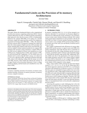
ICCAD ’20, November 2–5, 2020, Virtual Event, USASujan K. Gonugondla, Charbel Sakr, Hassan Dbouk, and Naresh R. Shanbhagclippedclipped(a)(a)(b)(c)Figure 3: Comparison of BGC and MPC: (a) MPC quantization levels, (b) BGC quantization levels, and (c) distribution𝑓𝑌 (𝑦o ) of the ideal DP output 𝑦o vs. DP dimensionality 𝑁 .Figure 4: Trends in SQNR𝑞 𝑦 (dB) for DP computation with𝐵𝑥 𝐵 𝑤 7: (a) SQNR𝑞 𝑦 (dB) vs. 𝑁 for MPC (𝜁 𝑦 4), BGC,if 𝑦o N (0, 𝜎 𝑦2 o ). The resulting SQNR𝑦 is given by:SQNR𝑞MPC𝑦 (dB)MPC 6𝐵 𝑦 4.8 𝜁 𝑦(dB)𝜎2 10 log10 1 𝑝 c 𝑐𝑐𝜎𝑞2𝑦(b)!(14) 𝑦22 E (𝑦 𝑦 ) 2 𝑦 𝑦 iswhere 𝜁 𝑦MPC 10 log10 𝜎 2c , and 𝜎𝑐𝑐ococ(dB)𝑦othe conditional clipping noise variance. Setting 𝑦c 𝜁 𝑦MPC 𝜎 𝑦𝑜 yieldsMPC 10 log (𝜁 MPC ) 2 indicating that 𝑝 is a decreasing function𝜁 𝑦(dB)c10 𝑦of 𝜁 𝑦MPC . Thus, (14) has the same form as (1) with an additional (lastterm) clipping noise factor.MPC exploits a key insight (see Fig. 3(c)), which follows from theCentral Limit Theorem (CLT) – in a 𝑁 -dimensional DP computation(2), 𝜎 𝑦o grows sub-linearly (as 𝑁 ) as compared to the maximum 𝑦mwhich grows linearly with 𝑁 . Furthermore, (14) shows a quantizationvs. clipping noise trade-off controlled by the clipping level 𝑦c . Thistrade-off, illustrated in Fig. 3(c), is absent in BGC and tBGC, and iscritical to MPC’s ability to realize desired values of SQNR𝑞 𝑦 withsmaller values of 𝐵 𝑦 .Assuming 𝑦o N (0, 𝜎 𝑦2 o ), and substituting 𝑦c 4𝜎 𝑦o , and𝑝 c 0.001 into (14), we obtain the following lower bound: 𝛾 i1h𝐵 MPC SNRA(dB) 7.2 𝛾 10 log10 1 10 10(15)𝑦6in order for SNRA(dB) SNRT(dB) 𝛾. For instance, the choice 𝛾 0.5 dB yields 𝐵 MPC 16 SNRA(dB) 16.3 which corresponds𝑦to SQNRMPC SNRA(dB) 9 dB as discussed in Section 3.2.𝑦(dB)tBGC, and (b) SQNR𝑞MPCvs. 𝜁 𝑦MPC when 𝐵 𝑦 8.𝑦 (dB)3.5Simulation ResultsTo illustrate the difference between MPC, BGC and tBGC, we assume that SNRa(dB) 31 dB, so that SNRT(dB) 30 dB providedSQNR𝑞𝑖𝑦 (dB), SQNR𝑞 𝑦 (dB) 40 dB per (10)-(11). We further assumeDPs of varying dimension 𝑁 with 7-b quantized unsigned inputsand signed weights randomly sampled from uniform distributions.Substituting 𝐵𝑥 𝐵 𝑤 7, 𝜁𝑥(dB) 1.3 dB, and 𝜁 𝑤(dB) 4.8 dBinto (8), we obtain SQNR𝑞𝑖𝑦 (dB) 41 dB. Thus, all that remains is toassign 𝐵 𝑦 such that SQNR𝑞 𝑦 (dB) 40 dB, for which there are threechoices - MPC, BGC and tBGC.Figure 4(a) compares the SQNR𝑞 𝑦 achieved by the three methods.Per (15), MPC meets the SQNR𝑞 𝑦 (dB) 40 dB requirement by set-ting 𝐵 𝑦 8 and 𝜁 𝑦MPC 4 independent of 𝑁 . In contrast, per (12),BGC assigns 16 𝐵 𝑦 20 as a function of 𝑁 to achieve the sameSNRT as MPC. Furthermore, tBGC meets the SQNR𝑞 𝑦 requirementwith 11 𝐵 𝑦 13 but fails to do so with 𝐵 𝑦 8. Figure 4(b)shows that SQNR𝑞MPCis maximized when 𝜁 𝑦MPC 4, i.e., when(dB)𝑦clipping level 𝑦c 4𝜎 𝑦o thereby illustrating MPC’s quantization vs.clipping noise trade-off described by (14). Figure 4 also validatesthe analytical expressions (8), (9), (13), and (14) (bold) by indicating

Fundamental Limits on the Precision of In-memory ArchitecturesICCAD ’20, November 2–5, 2020, Virtual Event, USATable 1: A Taxonomy of IMCs using In-memory ComputeModelsBeyond CMOSCMOSIn-memoryCompute ModelQS ISQRKang et al. [15]Biswas et al. [1]Zhang et al. [40]Valavi et al. [33]Khwa et al. [16]Jiang et al. [12]Si et al. [30]Jia et al. [11]Okumura et al. [23]Kim et al. [17]Guo et al. [8]Yue et al. [38]Su et al. [32]Dong et al. [4]Si et al. [31]Chen et al. [2]Fick et al. [5]Xue et al.[35]Yan et al.[37]Zha et al.[39]Xue et al.[36]Analog 81111151T115142TA3114ADCPrecision𝐵 ADC871113.465881355453A4116T: Ternary; A: Analog/Continuous-valueda close match to ensemble-averaged values of SQNR𝑞 𝑦 obtainedfrom Monte Carlo simulations (dotted).Note: the theoretically optimal quantizer given an arbitrary signal distribution is obtained from the Lloyd-Max (LM) algorithm[18]. Unfortunately, the LM quantization levels are non-uniformlyspaced which makes it hard to design efficient arithmetic units toprocess such signals. MPC offers a practical alternative to LM.4ANALYTICAL MODELS FOR COMPUTE SNRThis section derives analytical expressions for SNRa of a typicalIMC. First, we show that most IMCs can be ’explained’ via a fewin-memory compute models.4.1𝑉"" 𝑉 𝜙&In-memory Compute ModelsAll IMCs are viewed as employing one or more in-memory computemodels defined as a mapping of algorithmic variables 𝑦o , 𝑥 𝑗 and 𝑤 𝑗in (2) to physical quantities such as time, charge, current, or voltage,in order to (usually partially) realize an analog BL computation ofthe multi-bit DP in (2).Furthermore, we suggest that most IMCs today employ one ormore of the following three in-memory compute models (see Fig. 5):(a) charge summing (QS) [7, 14, 15, 40]; (b) current summing (IS)[12, 16, 17, 30]; and (c) charge redistribution (QR) [1, 7, 15, 33], andconjecture that these compute models are in some sense universal inthat they represent an approximation to a ‘complete set’ of practical,i.e., realizable, mappings of variables from the algorithmic to thecircuit domain as shown in Table 1.Henceforth, we discuss the QS model and the corresponding QSbased IMC referred to as QS-Arch in detail since it is very commonlyused. Analytical expressions for circuit domain equivalents of 𝜂 e𝑇&𝐼&𝜙&𝑉'𝑉)𝜙'𝑇'𝐺 𝑉"𝐺'𝐺)𝜙'𝐼'𝜙(𝑉 )(b)𝑉&𝜙"𝜙#𝑉"𝐶"𝜙 𝑉#𝐶#𝑉 𝐶 (c)Figure 5: In-memory compute models: (a) charge summing(QS), (b) current summing (IS), and (c) charge redistribution(QR) models.and 𝜂 h in (6) for the QS model are presented. These will be combinedwith algorithm and precision-dependent noise sources 𝑞𝑖𝑦 and 𝑞 𝑦to obtain SNRT .4.2The Charge Summing (QS) ModelThe QS model (see Fig. 5(a)) realizes the DP in (2) via the variablemapping (𝑦o 𝑉o , 𝑤 𝑗 𝐼 𝑗 , 𝑥 𝑗 𝑇 𝑗 ) where the cell current 𝐼 𝑗 isintegrated over the WL pulse duration 𝑇 𝑗 (𝑗 1, . . . , 𝑁 ) on a BL (orcell) capacitor 𝐶 resulting an output voltage as shown below:(𝑦o 𝑉o ) 𝑁1Õ(𝑤 𝑗 𝐼 𝑗 )(𝑥 𝑗 𝑇 𝑗 )𝐶 𝑗 1(16)where 𝑉o is the DP output assuming infinite voltage head-room,i.e., no clipping. The cell current 𝐼 𝑗 depends upon transistor sizesand the WL voltage 𝑉WL , and typical values are: 𝐶 (a few hundredfFs), 𝐼 𝑗 (tens of 𝜇As), and 𝑇 𝑗 (hundreds of ps).Noise Models: The noise contributions in QS arise from the following sources: (1) variations in the pulse-widths 𝑇 𝑗 of currentswitch pulses 𝜙 𝑗 (Fig. 5(a)); (2) their finite rise and fall times (seeFig. 6(b)); (3) spatial variations in the currents 𝐼 𝑗 ; (4) thermal noisein the discharge RC-network; and (5) clipping due to limited voltage head-room. Thus, the analog DP output 𝑉a corresponding to𝑦a 𝑦o 𝜂 a is given by:(𝑦𝑎 𝑉a ) (𝑦o 𝑉o ) (𝜂 e 𝑣 e ) (𝜂 h 𝑣 c ),𝑁1Õ𝑣 e 𝑣𝜃 𝑖 𝑗 𝑇 𝑗 𝐼 𝑗 (𝑡 𝑗 𝑡 rf ),𝐶 𝑗 1 𝑣 c min 𝑉o, 𝑉o,max 𝑉o,(17)

ICCAD ’20, November 2–5, 2020, Virtual Event, USASujan K. Gonugondla, Charbel Sakr, Hassan Dbouk, and Naresh R. Shanbhag𝐱" !𝑉 %𝑉# 𝐼" 𝐰!𝐱" "!𝑇!𝑤" ","𝑥 𝑤"!,#𝑥%𝐶 𝐰%!𝑥!𝑇"𝑇%𝐱" 𝟐𝑤" ", 𝐰% "&BLB𝑥&(b)ADCFigure 6: Modeling the discharge process in the QS computemodel: (a) cell current 𝐼 𝑗 , and (b) the word-line voltage pulse𝑉WL .ValueParameterValue𝑘 ′ (𝜇A/V2 )𝜎𝑇 0 (ps)Δ𝑉BL,max (V)𝑉t (V)𝑇 (K)2202.30.8-to-0.90.4270𝛼𝜎𝑉t (mV)𝑉WL (V)𝑇0 (ps)𝑘 (JK 1 )1.823.80.4-to-0.81001.38e-23𝑗 𝛼𝜎𝑉t 𝐼 𝑗 𝜎D𝑉WL 𝑉t 𝑉 𝑉 𝑇 𝑇trf𝑡 rf 𝑇𝑟 WL𝑉WL𝛼 1rq𝑘𝑇𝜎𝑇𝑗 ℎ 𝑗 𝜎𝑇 0, 𝜎𝜃 𝐶WLADCADC𝑦! ADCPOTS𝑦'Figure 7: The charge summing IMC (QS-Arch).𝐸 QS E [𝑉a ] 𝑉dd𝐶 𝐸 sucurrent mismatch, and 𝑡 𝑗 N (0, 𝜎𝑇2 ) is the noise due to (temporal)𝑗pulse-width mismatch, respectively, both of which are modeledas zero mean Gaussian random variables, 𝑡 rf models the impactof finite rise and fall times of the current switching pulses, and𝑣𝜃 N (0, 𝜎𝜃 ) is the thermal noise. Note: 𝑉o,max can be as high as0.9 V when 𝑉dd 1 V.Analytical expressions to estimate the noise standard deviations𝜎𝐼 𝑗 , 𝜎𝑇𝑗 , 𝜎𝜃 , and 𝑡 rf , (see appendix) are provided below: 𝐰% "&Energy and Delay Models: The average energy consumption inthe QS model is given by:where 𝑉o,max is the maximum allowable output voltage, and 𝑣 e and𝑣 c are the voltage domain noise due to circuit non-idealities andclipping, respectively, 𝑖 𝑗 N (0, 𝜎𝐼2 ) is the noise due to (spatial)𝜎𝐼 𝑗 𝐼 𝑗 POTSTable 2: QS Model Parameters in a 65 nm CMOS ProcessParameter𝑤" ",% Δ𝑉'(time(a) 𝑉'' 𝑉) BL 𝐰'𝐰%!(18)(19)(20)2 is normalized current mismatch variance, 𝑇 ℎ 𝑇 iswhere 𝜎D𝑗𝑗 0the delay of a ℎ 𝑗 -stage WL driver composed unit elements withdelay 𝑇0 each, 𝜎𝑇 0 is the standard deviation of 𝑇0 , 𝑇r and 𝑇f are WLpulse rise and fall times (see Fig. 6(b)), 𝛼 is a fitting parameter in the𝛼-law transistor equation, 𝜎𝑉t is standard deviation of 𝑉t variations,𝑘 is the Boltzmann constant, and 𝑇 is the absolute temperature.Note that typically the WL voltage 𝑉WL is identical for all rowsin the memory array with a few exceptions such as [40] whichmodulate 𝑉WL to tune the cell current 𝐼 𝑗 . The effects of rise/falltimes and delay variations can be mitigated by carefully designingthe WL pulse generators. Therefore, noise in QS is dominated byspatial threshold voltage variations. Indeed, using the typical valuesfrom Table 2, we find that 𝜎𝐼 𝑗 /𝐼 𝑗 ranges from 8% to 25%, while 𝜎𝑇𝑗 /𝑇 𝑗ranges from 0.5% to 3%.(21)where the spatio-temporal expectation E [𝑉a ] is taken over inputs(temporal) and over columns (spatial) 𝐸 su is the energy cost oftoggling switches 𝜙 𝑗 s. Equation (21) shows that the energy consumption in the QS model increases with 𝐶 array size, the supplyvoltage 𝑉dd , and the mean value of the DP E [𝑉a ].The delay of the QS model is given by 𝑇QS 𝑇max 𝑇su, where 𝑇suis the time required to precharge the capacitors and setup currents,and 𝑇max max{𝑇 𝑗 } is the longest allowable pulse-width.Table 2 tabulates parameters of the QS model in a representative65 nm CMOS process.4.3QS-ArchThe charge summing architecture (QS-Arch) in Fig. 7(b) employs a6T [8] or 8T [30] SRAM bitcell within the QS model (see Section 4.2).This architecture implements fully-binarized DPs on the BLs bymapping the input bit 𝑥ˆ𝑖,𝑗 to the WL access pulse 𝑉WL,𝑗 while theweights 𝑤ˆ 𝑖,𝑗 are stored across 𝐵 𝑤 columns of the BCA so that the BCcurrents 𝐼𝑖,𝑗 𝑤ˆ 𝑖,𝑗 . The output 𝑉o Δ𝑉BL is the voltage dischargeon the BL and the capacitance 𝐶 𝐶 BL is the BL capacitance in (16).QS-Arch sequentially (bit-serially) processes one multi-bit inputvector x in 𝐵𝑥 in-memory compute cycles followed by a digitalsumming of the binarized DPs to obtain the final multi-bit DP (2).Table 3 summarizes the noise and energy models for QS-Arch.We derive the analytical expressions of architecture-level noisemodels for QS-Arch using those of the QS model described in Section 4.2. In QS-Arch, clipping occurs in each of the 𝐵𝑥 𝐵 𝑤 binarizedDPs and contributes to the overall clipping noise variance 𝜎𝜂2h atthe multi-bit DP output. Circuit noise from each binarized DP isaggregated to obtain the final circuit noise variance 𝜎𝑒2 . In addition, employing MPC imposed requirement on the final DP outputprecision 𝐵 𝑦 (15), we obtain the lower bound on ADC precision𝐵 ADC .Since the multi-bit DP computation in (2) is high-dimensional(𝑁 can be in hundreds), it is clear that the limited BL dynamicrange e.g., 𝑉o,max in (17), will begin to dominate SNRa in (7). It isfor this reason that most, if not all, IMCs resort to some form ofbinarization of the multi-bit DP in (2) prior to employing one of thein-memory compute models (see Table 1). Ultimately, SNRa limits

Fundamental Limits on the Precision of In-memory ArchitecturesICCAD ’20, November 2–5, 2020, Virtual Event, USATable 3: Model Parameters for QS-ArchBitcell type6T or 8TAnalog Core PrecisionEnergy cost per DP𝐸 QS-Arch 𝐵 𝑤 𝐵𝑥 (𝐸 QS 𝐸 ADC ) 𝐸 miscCompute modelmapping𝜎𝑞2𝑖𝑦12 212 𝑁 Δ𝑥 𝜎 𝑤𝜎𝜂2e𝑁 𝜎D2 1 𝑁 Δ2 E 𝑥 2 12𝑤𝜎𝜂2h𝐵𝑥 1, 𝐵 𝑤 1𝐶 𝐶 BL𝑉o Δ𝑉BL𝑇 𝑗 𝑇WL,𝑗 4 1 4 𝐵 𝑤1 4 𝐵𝑥9 𝑘 3 𝑁 𝑘Í𝑁(𝑘 𝑘 h ) 2 𝑁𝑘 144𝑘 𝑘h(1 4 𝐵 𝑤)(91 4 𝐵𝑥)𝐵 ADC min SNRA(dB) 16.2, log2 (𝑘 h ), log2 (𝑁 )6𝜎𝐼BL.max𝑘 h Δ𝑉Δ𝑉BL,unit ; 𝜎D 𝐼 is the normalized standard deviation of the bit-cell current (18); (𝑥) max(𝑥, 0).component levelMonte Carlomeasurements fromDIMA prototypeSPICEsimulationsarchitecturemodelnoise modelsSNR expressionsSNR "non-linearbehavioral modelsample-accurate SNR !Python simulation SNRSNR !comparison"Figure 8: SNR validation methodology.the number and accuracy of BL computations per read cycle andhence the overall energy efficiency of IMCs.5SIMULATION RESULTSThis section describes the noise model validation methodology forvalidating the noise expressions in Table 3 and simulation resultsfor QS-Arch.5.1Noise Model Validation MethodologyFigure 8, we obtain the QS model parameters (Section 4) usingMonte Carlo circuit simulations in a representative 65 nm CMOSprocess, with experimental validation of some of these, e.g., 𝜎𝜂e ,from our IMC prototype ICs [6, 15] when possible.Incorporating non-linear circuit behavior along with noise models, sample-accurate Monte Carlo Python simulations are employedto numerically calculate SNR values using ensemble averaged (over1000 instances) statistics. We compare the SNR values obtainedthrough sample-accurate simulations with those obtained by evaluating the analytical expressions in Table 3.The quantitative results in subsequent sections employ the QSmodel parameter values in Table 2 along with QS-Arch energyand noise models from Table 3. An SRAM BCA with 512 rows and𝐶 BL 270 fF is assumed throughout. Energy and accuracy of QSArch is traded-off by tuning 𝑉WL . We assume zero mean signedweights 𝑤 𝑗 and unsigned inputs 𝑥 𝑗 drawn independently from twodifferent distributions. We set 𝐵𝑥 𝐵 𝑤 6 everywhere, unlessotherwise stated, so that SQNR𝑞𝑖𝑦 (dB) 38.9 dB SNRa(dB) andtherefore SNRA SNRa from (10). Next, we show how SNRA andSNRT trade-off with 𝑁 and 𝐵 ADC .5.2SNR Trade-offs in QS-ArchFigure 9(a) shows that the maximum achievable SNRA increaseswith 𝑉WL . Further, for a fixed 𝑉WL , QS-Arch also exhibits a sharpdrop in SNRA at high values of 𝑁 𝑁 max , e.g., SNRA 19.6 dB for𝑁 125 and then drops with increase in 𝑁 . A key reason for thistrade-off is that 𝜎𝜂2h decreases while 𝜎𝜂2e increases as 𝑉WL is reduced(see Table 3), and since 𝜎𝜂2h limits 𝑁 and 𝜎𝜂2e limits SNRa . Thus, bycontrolling 𝑉WL , we can trade-off 𝑁 max with SNRA . Specifically,𝑁 max increases by 2 for every 3 dB drop in SNRA .In QS-Arch, the minimum value of 𝐵 ADC (see Table 3) dependsupon the minimum of: 1) the MPC term (15); 2) the headroomclipping term; and 3) the small 𝑁 case where BL discharge Δ𝑉BL hasa finite number of discrete levels. Figure 9(b) shows that SNRT SNRA of Fig. 9(a) when 𝐵 ADC is greater than the lower bound(circled) in Table 3 for different values of 𝑉WL and 𝑁 .5.3Impact of ADC PrecisionMinimizing the column ADC energy is c

3 COMPUTE SNR LIMITS OF IMCS We propose the system noise model in Fig. 1 for obtaining precision limits on IMC architectures. Such architectures (Fig. 1(a)) accept a quantized input (x ) and a quantized weight vector (w ) to imple-ment multiple FX DP computations of (4) in parallel in its analog core.