Transcription
Application NoteChemical AnalysisSignal, Noise, and Detection Limits inMass SpectrometryAuthorsGreg Wells, Harry Prest, andCharles William Russ IV,Agilent Technologies, Inc.AbstractIn the past, the signal-to-noise of a chromatographic peak determined from a singlemeasurement has served as a convenient figure of merit used to compare theperformance of two different MS systems. Design evolution of mass spectrometryinstrumentation has resulted in very low noise systems that have made thecomparison of performance based upon signal-to-noise increasingly difficult, and insome modes of operation impossible. This is especially true when using ultra‑lownoise modes such as high resolution mass spectrometry or tandem MS; wherethere are often no ions in the background and the noise is essentially zero. Statisticalmethodology commonly used to establish method detection limits for trace analysisin complex matrices as a means of characterizing instrument performance is shownto be valid for high and low background noise conditions.
IntroductionTrace analysis in analytical chemistry generally requiresestablishing the limit of detection (LOD, or simply detectionlimit), which is the lowest quantity of a substance that can bedistinguished from the system noise absent of that substance(a blank value). Mass spectrometers are increasing usedfor trace analysis, and an understanding of the factors thataffect the estimation of analyte detection limits is importantwhen using these instruments. There are a number ofdifferent detection limits commonly used. These include theinstrument detection limit (IDL), the method detection limit(MDL), the practical quantification limit (PQL), and the limitof quantification (LOQ). Even when the same terminologyis used, there can be differences in the LOD according tonuances of what definition is used and what type of noisecontributes to the measurement and calibration. There ismuch confusion regarding figures of merit for instrumentperformance such as sensitivity, noise, signal-to-noiseratio and detection limits. An understanding of the factorsthat contribute to these figures of merit and how they aredetermined is important when estimating and reportingdetection limits. Modern mass spectrometers, which canoperate in modes that provide very low background noise andhave the ability to detect individual ions, offer new challengesto the traditional means of determining detection limits.Terminology– Instrument background signal—The signal output fromthe instrument when a blank is measured; generally avoltage output that is digitized by an analog to digitalconverter.– Noise (N)—The fluctuation in the instrument backgroundsignal; generally measure as the standard deviation of thebackground signal.– Analyte signal (S)—The change in instrument response tothe presence of a substance.– Total instrument signal—The sum of the analyte signaland the instrument background signal.– Signal-to-noise ratio (S/N)—The ratio of the analyte signalto the noise measured on a blank.– Sensitivity—The signal response to a particular quantityof analyte normalized to the amount of analyte givingrise to the response; generally determined by theslope of the calibration curve. Sensitivity is often usedinterchangeably with terms such as S/N and LOD. For thepurpose of this document, sensitivity will only apply to thisanalytical definition.2Instrument detection limit (IDL)Most analytical instruments produce a signal even whena blank (matrix without analyte) is analyzed. This signal isreferred to as the instrument background level. Noise isa measure of the fluctuation of the background level. It isgenerally measured by calculating the standard deviationof a number of consecutive point measurements of thebackground signal. The instrument detection limit (IDL) isthe analyte concentration required to produce a signal thatis distinguishable from the noise level within a particularstatistical confidence limit. Approximate estimate of LOD canbe obtained from the signal‑to-noise ratio (S/N) as describedin this document.Method detection limit (MDL)For most applications, there is more to the analytical methodthan just analyzing a clean analyte. It might be necessaryto remove unwanted matrix components, extract andconcentrate the analyte, or even derivatize the analyte forimproved chromatography or detection. The analyte mayalso be further diluted or concentrated prior to analysis onan instrument. Additional steps in an analysis add additionalopportunities for error. Since detection limits are defined interms of error, this will increase the measured detection limit.This detection limit (with all steps of the analysis included) iscalled the MDL. An approximate estimate of LOD can often beobtained from the S/N of the analyte measured in matrix.Limit of quantification (LOQ) and practical limit ofquantification (PQL)Just because we can tell something from noise does notmean that we can necessarily know how much of thematerial there actually is with a particular degree of certainty.Repeated measurements of the same analyte under thesame conditions, even on the same instrument, give slightlydifferent results each time due to variability of sampleintroduction, separation, and detections processes in theinstrument. The LOQ is the limit at which we can reasonablytell the difference between two different values of the amountof analyte. The LOQ can be drastically different betweenlabs so another detection limit referred to as the PracticalQuantitation Limit (PQL) is commonly used. There is nospecific mathematical relationship between the PQL and theLOQ based on statistics. The PQL is often practically definedsimply as about 5 to 10 times the MDL.
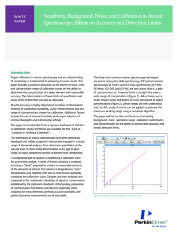
Estimating IDL and MDL using signal‑to-noiseMass spectrometry measurements of an analyte generallyuse a chromatograph as a means of sample introduction.The resulting analyte signal from a chromatograph will havean approximately Gaussian shaped distribution as a functionof time (Figure 1). In the case of chromatographic analyteintroduction into the MS instrument, the signal is not constantand does not represent the same analyte amount at all pointsof the sample set. For the purpose of estimating detectionlimits by using signal-to-noise ratios, the measurement of thesignal is generally accepted to be the height of the maximumof the chromatographic signal (S in Figure 1) above thebaseline (ΧB), and an estimate of the background noise underthe peak must be made. A standard for estimating the noiseis to measure the peak-to-peak (minimum to maximum)value of baseline noise, away from the peak tails, for 60seconds before the peak (Figure 1) or 30 seconds beforeand after the peak. With the advent of modern integrator anddata systems, the baseline segments for estimation of noiseare auto‑selected, and noise is calculated as the standarddeviation (STD) or root-mean-square (RMS) of the baselineover the selected time window. However, it will be shown thatthe single measurement S/N approach fails in many cases.SignalSXBTimeStartEndFigure 1. Analyte signal as a function of time for a chromatographic peak,demonstrating the time dependence in the amount of analyte present.When a quantitative measurement of the amount of analyte ismade, the signal is the total integrated signal of the Gaussianpeak from start to end with the background subtracted. Thisarea is a single sampling measurement and is a single pointestimator for the true analyte amount in the population (thatis, the amount of analyte in the original sample). The amountof analyte as a function of time can be expressed as: C(t) KC0F(t); where C0 is the amount of analyte in the test sample,F(t) is the shape of the chromatographic peak (amplitudeversus time), and K is a calibration factor. If the analyte profileis reproducible and the response is linear in analyte amount,the area of the peak can be used as a measure of the originalamount of analyte since the constant of proportionality, K,can be determine by calibration using known amounts ofanalyte. Repeated measurements (areas) of the same samplewill yield a set of somewhat different responses that arenormally distributed about the true value representing thepopulation. The variance in the measured set of signals forboth the sample and the background are due to a variety offactors: (1) variances in the amount injected, (2) variancesin the amount of sample transferred onto the GC column,(3) variances in the amount of background, (4) variances inthe ionization efficiency, (5) variances in the ion extractionfrom the ion source and transmission through the massanalyzer, and (6) variances in the recorded detection signalrepresenting the number of ions measured. The latter factorat low ion fluxes will occur even if the number of ions strikingthe ion detector were the same, the output signal will beslightly different since the ion detector response depends onwhere the ion strikes it. A significant contributor to variancewill be the determination of the area of the chromatographicpeak. Variations in the determination of peak start, end andarea below the background all contribute errors. Collectively,these variances can be viewed as sampling noise. That is,variations in the output signal due to the collective samplingand detecting processes. These variances are in addition tothe normal variations due to measuring a finite number ofions (that is, the ion statistics).Modern mass spectrometer systems are capable of operatingin a variety of modes that can make the backgroundnearly zero. MS/MS, negative ion chemical ionization,and high resolution mass scanning can often have a nearzero system background signal, particularly when thebackground from a chemical matrix is absent. Figure 2shows a GC/MS extracted ion chromatogram for a cleanstandard of octafluoronaphthalene (OFN) in a clean systemwith a very low background. Each point in an extracted ionchromatogram represents the intensity of a centroided masspeak. If there are not enough ions for a particular mass tobe centroided, the resulting intensity value may be reportedas zero. It is possible with very clean systems operating inthe MS/MS or negative chemical ionization mode to haveno observable background ions and a zero calculated noise.This situation can be made more severe by increasing thethreshold for ion detection. Under these circumstances, it ispossible to increase the ion detector gain, and the signal level,without increasing the background noise. The signal of theanalyte increases, but the noise does not. This is misleadingand unacceptable.3
9,000272.00 m/z8,000Abundance7,0006,0005,0004,0003,0002,000(a )(b )(c)1,00004.04.44.85.25.66.06.46.8Time (min)Figure 2. EI full scan extracted ion chromatogram of m/z 272 from 1 pg OFN exhibiting verysmall chemical ion noise.The result is two practical problems: (1) What region of thebaseline should be selected to estimate the backgroundnoise, and (2) although the signal increased, there was noincrease in the number of ions detected and therefore nochange to the real detection limit. Unlike the high backgroundcase, when the background is very low, but not zero, themeasured noise will depend strongly on where the noise ismeasured. The regions of the background labeled (a), (b), and(c) in Figure 2 have measured RMS noise values that are 54,6, and 120 respectively. The resulting S/N values can differby a factor of 20 in this example due exclusively to the largevariation in where the noise is measured. Therefore, the useof S/N as an estimate of the detection limit will clearly fail toproduce usable values when there is low and highly variableion noise. The situation becomes even more indeterminatewhen the background noise is zero as shown in the MS/MSchromatogram in Figure 3. In this case, the noise is zero andthe S/N becomes infinite. The only noise observed in Figure 3is due to the electronic noise, which is several orders ofmagnitude lower than noise due to the presence of ions in thebackground.9,000272 m/z & 222 me (min)Figure 3. EI MS/MS extracted ion chromatogram of m/z 222.00 from 100 fg OFN exhibiting nochemical ion noise.4
Alternate methods to estimating IDL and MDLThere are many alternative methods to estimate the IDL andMDL that produce more reliable estimates2–7 for analytesintroduced by a chromatograph. For the USA, the mostcommon is the recommended EPA Guidelines EstablishingTest Procedures for the Analysis of Pollutants.2 A commonlyused standard in Europe is found in The Official Journal of theEuropean Communities, Commission Decision of 12 August2002; Implementing Council Directive 96/23/EC concerningthe performance of analytical methods and the interpretationof results.4Both of these methods are similar and require injectingmultiple duplicate standards to assess the uncertainty inthe measuring system. A small number of identical sampleshaving a concentration near the expected limit of detection(within 5 to 10 times the noise level) are measured along witha comparable number of blanks. The average blank valueis subtracted from each of the analyte measurements toremove the area contribution from any constant backgroundif necessary. Often, because of the specificity of massspectrometry detection, the contribution from the blankis negligible and is excluded once the significance of thecontribution has been confirmed. The standard deviationof the set of measured analyte signals (that is, integratedareas of the baseline subtracted chromatographic peaks)is then determined. Since the variance in the peak areasincludes both the analyte signal noise, the background noise,and the variance from injection to injection; the statisticalsignificance of a single measurement being distinguishablefrom the system and sampling noise can be establishedwith a known confidence level (that is, a known probabilitythat the measured area is statistically different from thesystem noise). The use of signal-to-noise from a singlesample measurement as an estimate of IDL does not capturethe sample-to-sample variation or sampling noise thatcauses multiple measurements of the same analyte to besomewhat different.When the number of measurements is small (that is n 30),the one‑sided Student t-distribution1 is used to determinethe test statistic tα. In the case of chromatographic peaks,modern data systems report the area of the peak above thebaseline, (that is, the background is subtracted, but not thecontribution to the variance of the signal). The IDL or MDLis determined as the amount of analyte Χ that gives a signal(peak area) statistically greater than the population meanvalue of zero (µ 0) as detailed in Appendix I.IDL Χ – µ Χ tασΧ tαSΧWhere the value of tα comes from a table of the Studentt-test using n – 1 (number of measurements minus one)as the degrees of freedom, 1 – α is the probability that ameasurement is greater than zero, and the standard deviationof the set of measurements SΧ is used as an estimate ofthe true standard deviation of the distribution of samplemeans. This discussion eatablishes that at least two or moremeasurements are required in order to estimate the standarddeviation and estimate the sampling noise. The larger thenumber of measurements n, the smaller is the value of tα andless the uncertainty in the estimate of the IDL or MDL.Figure 4 shows that for a given amount of standard, CSTD,replicate measurements produce a distribution of measuredvalues centered about the mean value ΧSTD. The standarddeviation is a measure of the width of this distribution. TheIDL is amount of sample, CIDL, corresponding to a meanmeasured value, ΧIDL , that allows 1 – α of the measurementsto be greater than zero; where α is the percentage orprobability that a measured value is equal or less than zero.Figure 5 shows the effect of a smaller standard deviation(greater precision) for the same α and the same instrumentsensitivity. A smaller standard deviation of the measurements,keeping α the same, results in a smaller IDL since the meanvalue of the measured distribution is moved to smaller valuesin order to keep the same percentage (that is, same α) of thenew distribution greater than zero.SignalStandarddeviationX STD–1X IDLAmountα–1C IDLC STDFigure 4. Instrument detection limit–amount of analyte with signal that isstatistically 0. Large variance in measured values.5
As an example, for the eight replicate injections in Figure 6(seven degrees of freedom; n 7) and a 99% (1 – α 0.99)confidence interval, the value of the test statistic (tα) is 2.998.Since the instrument detection limit is desired, a populationmean of zero is assumed (that is 99% probability that a singlemeasurement of ΧA (a single area measurement) will resultin a signal statistically greater than zero with a probability of1 – α). For eight samples, the mean value of the area is 810counts, the standard deviation is 41.31 counts, the relativestandard deviation is 5.1% and the value of the IDL is:SignalStandarddeviationX STDIDL tαSΧ–1X IDL–2X IDLAmountαC IDL–2 C IDL–1C STDFigure 5. Instrument detection limit–amount of analyte with signal that isstatistically 0. Small variance in measured values.500ΧA (2.998)(41.31) 123.85 counts. Since the calibrationmean for 200 fg was 810 counts, the IDL is: (123.85 counts)(200 fg)/(810 counts) 30.6 fg.For data systems reporting relative standard deviation (RST)the IDL is:IDL (tα)(RSD)(amount standard)/100%. In the previousexample the IDL (2.998)(5.1%)(200 fg)/100% 30.6 fg272.00 m/zPeak area 810 countsSTD 41.3 countsPeak area RSD 5.1%IDL 31 fg400Counts30020010008.08.18.28.3Time (min)Figure 6. EI full scan extracted ion chromatograms of m/z 272 from 200 fg OFN; eight replicate injections.68.4
ConclusionAppendix IThe historical use of the signal-to‑noise ratio of achromatographic peak determined from a singlemeasurement is a convenient means of estimating IDL inmany cases. A more practical means of estimating the IDLand MDL is to use the multi-injection statistical methodologycommonly used for trace analysis in complex matrices. Usingthe mean value and standard deviation of replicate injectionsprovides a way to estimate the statistical significance ofdifferences between low level analyte responses and thecombined uncertainties in both the analyte and backgroundmeasurement, and the uncertainties in the analyteintroduction or sampling process. This is especially truefor modern mass spectrometers for which the backgroundnoise is nearly zero. The multi-injection method of estimatinginstrument and method detection limits is rigorously andstatistically valid for both high and low background noiseconditions.How a signal is distinguished from noiseReferences1. Statistics; D. R. Anderson, D. J. Sweeney, T. A. Williams;West Publishing, New York, 1996.2. U.S. EPA - Title 40: Protection of Environment; Part 136–Guidelines Establishing Test Procedures for the Analysisof Pollutants; Appendix B to Part 136 – Definition andProcedure for the Determination of the Method DetectionLimit – Revision 1.11.3. Uncertainty Estimation and Figures of Merit forMultivariate Calibration; IUPAC Technical Report. PureAppl. Chem. 2006, 78(3), 633–661.4. Official Journal of the European Communities;Commission Decision of 12 August 2002; ImplementingCouncil Directive 96/23/EC concerning the performanceof analytical methods and the interpretation of results.5. Guidance Document on Residue Analytical Methods;European Commission – Directorate General Health andConsumer Protection; SANCO/825/00 rev. 7 17/03/2004.6. Guidelines for Data Acquisition and Data QualityEvaluation in Environmental Chemistry - ACS Committeeon Environmental Improvement. Anal. Chem. 1980, 52,2242–2249.7. Guidlines for the Validation of Analytical Mrthodsused in Residue Depletion Studies; VICH GL 49(MRK) – November 2009 Doc. Ref. EMEA/CVMP/VICH/463202/2009-CONSULTATION.The estimation of detection limits depends on how a signalfrom an analyte is distinguished from the background noise.The methodology for this estimate is rooted in statisticalhypothesis testing. Hypothesis testing is similar to a criminaltrial. In a criminal trial, the assumption is that the defendantis innocent. The null hypothesis H0, expresses an assumptionof innocence. The opposite of the null hypothesis is Ha, thealternative hypothesis – it expresses an assumption of guilt.The hypothesis for a criminal trial would be written:H0: The defendant is innocentHa: The defendant is guiltyTo test these competing statements, or hypothesis, a trialis held. The evidence presented at trail provides the sampleinformation. If the sample information is not inconsistentwith the assumption of innocence, the null hypothesis thatthe defendant is innocent cannot be rejected. However, ifthe sample information is inconsistent with the assumption,the null hypothesis must be rejected and the alternativehypothesis can be accepted.In the case of chromatographic peaks, modern data systemsreport the area of the peak above the baseline (that is, theconstant background is subtracted, but not the contribution tothe variance of the signal). The mean value of the populationµA of the analyte is the true value of the amount of analytestored in the analyte collection vessel. A measurement of asample aliquot is a single‑point estimation of the populationmean. The mean value ΧA of a set of replicate samplemeasurements is an approximation to the population meanµA. The question to be answered: Is the sample set meanvalue statistically greater or equal to the mean populationwithin some specified confidence level? Since the IDL isdesired, the population mean is assumed to be zero. In thiscase the rejection criterion is:– H0: µA 0 The estimate of the signal is not different fromzero within the stated confidence or significance limit.– Ha: µA 0 The estimate of the signal is different from zerowithin the stated confidence or significance limit.– Accept H0 if µA 0 and reject H0 if µA 0 and accept thealternative hypothesis Ha.7
The statistical criteria for testing the hypothesis is: if thetest statistic tα is less than a value that is obtained from aprobability table. The table value depends on the number ofmeasurements (n) that contributed to obtaining the meanvalue and the probability that the mean value is greater thanthe population mean.tα Χ–µ table valueσΧWhere:ΧA is the mean value of the set of sample measurementsµA is the true value of the populationσΧ is the standard deviation of the set of samplemeasurementstα is the test statistic1 – α is the probability that the sample set mean is differentfrom the population meanwww.agilent.com/chemThis information is subject to change without notice. Agilent Technologies, Inc. 2011, 2021Printed in the USA, October 12, 20215990-7651ENThe value of the test statistic t depends on the numberof degrees of freedom which is defined as the numberof measurements minus one. For small numbers ofmeasurements (n 30), the value of tα comes from a tableof the Student t-test using n – 1 (number of measurementsminus one). For example, for seven measurements (sixdegrees of freedom) and a confidence level of 99% (α 0.01which is a 99% probability that the value is different from zero;µ 0) the table value is 3.143. Therefore, if:ΧΧ–µ t 3.143SΧ ασΧaccept the null hypothesis, and if this is greater than tα,the null hypothesis must be rejected and the alternativehypothesis (that is, the background corrected analyte signalis statistically different from zero) must be accepted with a1 – α probability of being correct. The value of the standarddeviation of the population σΧ is usually approximated by thestandard deviation of the sample set SΧ. For four samples(three degrees of freedom) and a 97.5% confidence level,the value of the test statistic is 3.18. For eight samples(seven degrees of freedom) and a 99.0% confidence level,the value of the test statistic is 2.90. The average value isapproximately 3. Therefore, the common rule for estimatingthe IDL or MDL is: ΧIDL 3 SΧ.
there are often no ions in the background and the noise is essentially zero. Statistical methodology commonly used to establish method detection limits for trace analysis in complex matrices as a means of characterizing instrument performance is shown to be valid for high and low background noise conditions. Signal, Noise, and Detection Limits in