Transcription
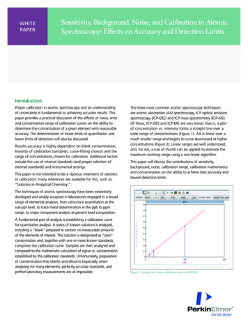
WHITEPAPERSensitivity, Background, Noise, and Calibration in AtomicSpectroscopy: Effects on Accuracy and Detection LimitsIntroductionProper calibration in atomic spectroscopy and an understandingof uncertainty is fundamental to achieving accurate results. Thispaper provides a practical discussion of the effects of noise, errorand concentration range of calibration curves on the ability todetermine the concentration of a given element with reasonableaccuracy. The determination of lower limits of quantitation andlower limits of detection will also be discussed.Results accuracy is highly dependent on blank contamination,linearity of calibration standards, curve-fitting choices and therange of concentrations chosen for calibration. Additional factorsinclude the use of internal standards (and proper selection ofinternal standards) and instrumental settings.This paper is not intended to be a rigorous treatment of statisticsin calibration; many references are available for this, such as“Statistics in Analytical Chemistry1".The three most common atomic spectroscopy techniquesare atomic absorption (AA) spectroscopy, ICP optical emissionspectroscopy (ICP-OES) and ICP mass spectrometry (ICP-MS).Of these, ICP-OES and ICP-MS are very linear; that is, a plotof concentration vs. intensity forms a straight line over awide range of concentrations (Figure 1). AA is linear over amuch smaller range and begins to curve downward at higherconcentrations (Figure 2). Linear ranges are well understood,and, for AA, a rule of thumb can be applied to estimate themaximum working range using a non-linear algorithm.This paper will discuss the contributions of sensitivity,background, noise, calibration range, calibration mathematicsand contamination on the ability to achieve best accuracy andlowest detection limits.The techniques of atomic spectroscopy have been extensivelydeveloped and widely accepted in laboratories engaged in a broadrange of elemental analyses, from ultra-trace quantitation at thesub-ppt level, to trace metal determination in the ppb to ppmrange, to major component analysis at percent level composition.A fundamental part of analysis is establishing a calibration curvefor quantitative analysis. A series of known solutions is analyzed,including a “blank” prepared to contain no measurable amountsof the elements of interest. This solution is designated as “zero“concentration and, together with one or more known standards,comprises the calibration curve. Samples are then analyzed andcompared to the mathematic calculation of signal vs. concentrationestablished by the calibration standards. Unfortunately, preparationof contamination-free blanks and diluents (especially whenanalyzing for many elements), perfectly accurate standards, andperfect laboratory measurements are all impossible.Figure 1. Example of a linear calibration curve in ICP-MS.
graphite furnace AA, based on a more thorough and widelyranging definition2. However, these procedures are specific towater, wastewater and other environmental samples.There are few widely accepted approaches for other matricessuch as food, alloys, geological and plant materials, etc. It is leftto the lab doing the analysis to establish an approach to answerthe question “How low a concentration of a given element canwe detect in a particular sample matrix?” Because there existsa long history in most labs and many different techniques areemployed (e.g., GC, LC, UV/Vis, FT-IR, AA, ICP, and many others)there are many opinions and approaches to this subject.Figure 2. Example of a non-linear calibration curve in AA.Detection Limits – “How Low Can We Go?”Under ideal conditions, the detection limits of the varioustechniques range from sub part per trillion (ppt) to sub part permillion (ppm), as shown in Figure 3. As seen in this figure, thebest technique for an analysis will be largely dependent on thelevels that need to measured, among other considerations.Detection Limit Ranges (μg/L)Figure 3. Detection limit ranges of the various atomic spectroscopy techniques.It is important to realize that detection limits are not the same asreporting limits: just because a concentration can be detected doesnot mean it can be reported with confidence. There are manyfactors associated with both detection limits and reporting limitswhich distinguish each, as will be seen in the following discussion.A discussion of detection limits can be lengthy and is subjectto many interpretations and assumptions – there are evenseveral definitions of “detection limits”. In atomic spectroscopy,there are some commonly accepted approaches. Under someanalytical protocols, the determination of detection limits isexplicitly defined in a procedure, as in U.S. EPA methods 200.7and 6010 for ICP, 200.8 and 6020 for ICP-MS, and 200.9 for2How, Then, Do We Establish “How Low We Can Go”?The simplest definition of a detection limit is the lowestconcentration that can be differentiated from a blank. The blankshould be free of analyte, at least to the limit of the techniqueused to measure it. Assuming the blank is “clean”, what is thelowest concentration that can be detected above the averageblank signal?One way to determine this is to first calibrate the instrumentwith a blank and some standards, calculate a calibration curve,and then attempt to measure known solutions as samples atlower and lower concentrations until we reach the point thatthe reported concentration is indistinguishable from the blank.Unfortunately, no measurement at any concentration is perfect– that is, there is always an uncertainty associated with everymeasurement in a lab. This is often called “noise”, and thisuncertainty has several components. (A detailed discussion ofsources of uncertainty is also a lengthy discussion3 and beyondthe scope of this document.) So, to minimize uncertainty, it iscommon to perform replicate measurements and average them.The challenge, then, is to find the lowest concentration that canbe distinguished from the uncertainty of the blank. This can beestimated by using a simple statistical approach. For example, U.S.EPA methods for water use such an approach. After calibration, ablank is run as a sample 10 times, the 10 reported concentrationsare averaged and the standard deviation is calculated. A test forstatistical significance is applied (the Student’s t-test) to calculatewhat the concentration would be that could be successfullydifferentiated from the blank with a high degree of confidence. Inthe U.S. EPA protocol, a 99% confidence is required. This equatesto three times the standard deviation of 10 replicate readings. Thisis also known as a 3σ (sigma) detection limit and is designated asthe Instrument Detection Limit (IDL) for U.S. EPA methods.It is important to note that the statistically calculated detectionlimit is the lowest concentration that could even be detected ina simple, clean matrix such as 1% HNO3 – it is not repeatable orreliable as a reported value in a real sample.To be more repeatable, the signal (with its associated uncertainty)must be significantly higher than the uncertainty of the blank,perhaps 5-10 times the standard deviation of the blank. This is ajudgment by the lab as to how confident the reported value shouldbe. This concentration level might be called the lowest quantitationlimit, sometimes known as PQL (practical quantitation limit), LOQ(limit of quantitation) or RL (reporting limit). There are no universallyaccepted rules for determining this limit.
Again, the EPA has guidelines in some methods for water samplesthat establish a lower reporting limit as a concentration that canbe measured with no worse than /- 30% accuracy in a preparedstandard. This rule is only applicable to the specific EPA methodand in water samples.Many labs apply the EPA detection limit methodologies simplybecause there are few commonly accepted and carefully definedapproaches for other sample types. Some industries followASTM, AOAC or other industry guidelines, and some of theseprocedures include lower-limit discussions.When analyzing a solid sample, the sample must first be broughtinto solution, which necessarily involves dilution. The estimationof detection or quantitation limits now needs to account for thedilution factor and matrix effects. For example, if 1 g of sample isdissolved and brought to a final volume of 100 mL, the detectionlimit in the solution must be multiplied by the dilution factor(100x in this example) to know what level of analyte in theoriginal solid sample could have been measured if it couldhave been analyzed directly.To use the statistical estimate technique (3σ detection limit), a“clean” matrix sample must be available, but this is not alwayspossible. The very product or incoming material being evaluatedmay be the best example available, but it may be contaminatedwith the element being determined – indeed, this is the purposeof the analysis. Finding a true “blank” is difficult.In many cases, then, a more empirical or practical approach istaken. After preparing the sample, it is spiked with a knownamount of analyte and measured. If the spike recovery isaccurate within some acceptable limits (this is also subjectto many opinions and there is no “rule” about what isacceptable accuracy, although the EPA has a rule for spikerecovery when analyzing environmental samples), then a lowerconcentration spike is attempted. After a series of lower andlower concentration spikes, there will be a point at which“confidence” is lost. The analyst would then set a limit forreporting that is at or above a level that gives reasonableaccuracy. This is a gray area and is up to the lab to decide.Again, a multiplier for dilution factor must be incorporated intothis reporting limit if the sample has been diluted for analysis.What factors are important for achieving the best possibledetection limits? They are:limits. For example, if contamination is present, a 10-fold increasein signal will also increase the background 10-fold. In an idealsituation (i.e. the absence of high background or excessive noise)detection limits theoretically improve by the square root of theincrease in signal intensity (i.e. a 9x increase in intensity will improvedetection limits 3x). However, as we will see, background level andnoise have as much of a contribution to detection limits as intensity.In ICP-OES and ICP-MS, a common way to express intensityis “counts per second”, or cps. We will use this unit in thefollowing discussion.Background Signal Plays an Important Role inDetection LimitsConsider an example with a signal that gives an easily measurableintensity of 1000 cps. However, if the background is 10,000 cpsthe signal is small relative to the background. It is common toexpress the relationship between signal and background as the“signal-to-background ratio” or S/B. (This is often referred to as“signal-to-noise” or S/N, but background and noise are two distinctcharacteristics). The above example would have an S/B of 0.1.However, if the background were only 1 cps, the same 1000 cpssignal would have a S/B of 1000, or 10,000 times better than thefirst example. These two examples are illustrated in Figure 4, whichshows that a smaller signal, say 100 cps, is easier to distinguishfrom a background of 1 cps than a background of 10,000 cps.All signals are measured in the presence of some degree ofbackground, which can originate from a variety of sources,including detector and electronic characteristics, emitted lightfrom the excitation source (prevalent in ICP-OES), interfering ionsformed in the source or from the matrix (prevalent in ICP-MS),or contamination. A quantitative measure of background levelis called the “Background Equivalent Concentration”, or BEC,which is defined as the concentration of a given element thatexhibits the same intensity as the background, measured at agiven wavelength (ICP-OES) or mass (ICP-MS). BEC is calculatedwith the following formula:BEC IblankCstandardIstandard - Iblank *Iblank Intensity of the blankIstandard Intensity of the standardCstandard Concentration of the standard1. Signal “strength” or sensitivityThe units of the BEC are the same as the units of the standard.2. BackgroundTo illustrate, consider an example of two elements, A and D.Suppose Element A has a sensitivity of 1000 cps/ppb, and elementD has a sensitivity of 10,000 cps/ppb. We would say that D has10 times more sensitivity than A. However, if the mass of D is thesame as a common background species produced in the argonplasma (such as ArO ), the background signal would be high(100,000 cps for ArO in this example). If Element A has nointerfering background species, the background could be1 cps, due only to electronic effects.3. Noise4. StabilityLet’s examine each of these.Sensitivity Plays a Role in Detection LimitsSignal strength (intensity) must be sufficient to differentiatethe presence of an element above the background AND noise;this is known as “sensitivity” and is an important characteristic.However, sensitivity is not, by itself, sufficient to predict detection3
Even though element D is 10x more sensitive, the ability to detect Dis worse than A, as shown in Figure 4. The BEC for A is 0.001 ppbwhile the BEC for D is 10 ppb. Note that BEC is NOT a detectionlimit, but an indicator of relative size of the signal from the elementand background. The lower the BEC, the lower the detection limit.At medium sensitivity, a Ho blank gives 0.2 cps, and a 1 ppbstandard gives 121,000 cps, which yields a BEC and detectionlimit of 0.002 ppt. With a 10x higher signal (1,270,000 cps) butno increase in blank, the BEC and detection limit improve to0.0002 ppt and 0.0007 ppt, respectively.Now consider the same situation for Pb, as shown in Table 2.Table 2. Lead at Medium and High Sensitivities.SampleMedium SensitivityHigh SensitivityBlank (cps)78701Standard (cps)Figure 4. Graphical representation demonstrating that a constant analyte signal(stripes) is more easily seen with a lower background signal (green).Another case is an element that normally has no backgroundcontribution above the instrument background of 1 cps –lead (Pb). In the example in Figure 5, the Pb background is100 cps,5due to Pb contamination. As a result, the Pb BECFigureand detection limits both increase, compared to an analysiswith no Pb contamination.1 ppt Pb 1% HNO3cps3001 ppt Pb2001001% HNO381000809000BEC (ppt)1.00.9DL (ppt)0.380.42In this example, there is Pb contamination in blank, so whensensitivity increases 10x, the signals in both the blank andstandard increase 10x, meaning the S/B remains constant. Asa result, there is no improvement in BEC or DL, despite theincrease in sensitivity. Since most elements measured by ICPMS have some interference or contamination on their masses,higher sensitivity does not always improve BEC or DLs.Noise Plays an Important Role in Detection LimitsIn the example above, the inherent assumption is that thesignal and the background are perfect measurements; thatis, 1000 cps has no variability, and the background has novariability. However, this is never the case in a real laboratorymeasurement: all measurements have uncertainty, which isreferred to as “noise”. For example, if a signal of 1000 cps wasmeasured five times, it would vary - 995, 1028, 992, 1036,987 cps. This is why replicate readings are measured: becausethey are never perfect, we want to measure multiple times andtake the average. In the above example, an average of the fivereadings (1008 cps) would be reported. How much variabilitythere is among the replicates would be indicated by using theStandard Deviation (for absolute variation) and/or the RelativeStandard Deviation (for a percentage). So, the reported value incps would be:1008 /- 20 cps (using the standard deviation)BEC of Pb 1pptorFigure 5. Relationship of BEC and DL on lead (Pb). Signal from Pb is in orange; thesignal from the background is blue.Now consider the effect of increased sensitivity on BEC anddetection limit for Pb and holmium (Ho). While Pb is a verycommon element, Ho is not. As a result, Pb contamination iscommon, while Ho contamination is rare. If there is no interferenceor contamination on an analyte mass, a 10x increase in sensitivityimproves the DL by a factor of 3 (the square root of the increase).In Table 1, Ho has two different sensitivities.Table 1. Holmium at Medium and High Sensitivities.SampleMedium SensitivityHigh SensitivityBlank (cps)0.20.2Standard (cps)41210001270000BEC (ppt)0.0020.0002DL (ppt)0.0020.00071008 /- 2% (using the relative standard deviation)Now superimpose “noise” or “uncertainty” on an example,assuming a signal of 1000 cps and a background of 10000 cps: If the signal of 1000 cps had an uncertainty of /- 2%, thenthe signal could be 980 – 1020 cps. If the background also had an uncertainty of 2%, then itsrange could be 9800-10200 cps.
Figure 6 shows an illustration of a small signal on top ofbackground noise.Figure 8On the left, a small analyte signal (blue) is “buried” in thenatural uncertainty of the high background and is difficultto see. In addition, the analyte signal has its own uncertainty.If the background is high relative to the analyte signal, theability to quantitate (or even detect) is compromised. On theright, the same analyte signal is easily differentiated from alow background. At very low concentrations near detectionlimits, longer integration times are necessary to average thenoise of both signals.Stability is Important For Reliable Detection LimitsStability plays a large role in detection limits in that small signalsmust be very steady to give valid noise averaging. The detectionlimit is the smallest signal that, on average, can be distinguishedfrom the average noise of the blank, as shown in Figure 6. It isimportant to note that the noise and stability are as importantas the absolute signal size in being able to differentiate a “real”signal from the noise of the blank.Furthermore, if an analytical sequence lasts for many minutesor hours, the baseline must be stable for small signals to bemeasured as accurately as statistical variation allows. Figure 7shows a blank analyzed repeatedly (after calibration, resultsin concentration units of mg/L). The variation would be called“noise”. Following the EPA protocol for estimating detectionlimit, the first 10 readings were averaged and the StandardDeviation calculated, giving a value of 0.0086 mg/L; threetimes the standard deviation (99% confidence level, Student-ttest) equals 0.025 mg/L. The red line in Figure 7 shows this 3σdetection limit for this analysis.However, if the analytical conditions are not stable over the timeframe of the sample run (i.e. batch of samples), the reportedresults can be well below the calculated detection limit. Figure 8shows the effect of drift: towards the end of the run, reportedconcentrations for a blank sample are as low as -0.05 mg/L.Therefore, a sample with as much as 0.075 mg/L would reportas “below detection limit” of 0.025 mg/L.Figure 7. Concentration measurements of a blank (blue line) and associated detectionlimit (red line), determined as three times the standard deviation of the blank.Concentra on (mg/L)Figure 6. Effect of background and noise on a small signal.Error of 0.075 mg/LSampleFigure 8. The reported concentration of a blank sample (blue line) decreases overtime due to instrument drift. During the final reading, the sample reads 0.075 mg/Lbelow the detection limit (red line).Calibration – Effects on Accuracy and Detection LimitsAll quantitative answers reported for a sample are calculatedfrom the calibration curve. Proper calibration is crucial foraccurate results AND ESPECIALLY for low-level results neardetection limits.A characteristic of atomic spectroscopy instrumentationis linearity: ICP-OES has a linear range of 5-6 orders ofmagnitude, while the linear range of ICP-MS is 10-11 ordersof magnitude. Statistically, these are accurate statements.However, consider a series of calibration standards from1 ppt to 1000 ppm (a range of 109 or nine orders ofmagnitude) analyzed by ICP-MS. The resulting calibrationcurve would be linear, giving a correlation coefficient (R2) of0.9999 or better (a perfect fit would have a correlation of1.000000). A common misunderstanding of this statistic isthat any concentration from 1 ppt to 1000 ppm could thenbe read accurately because the curve is “linear”.5
Figure 9Figure 9 shows an excellent linear relationship over six orders ofmagnitude (R2 0.999905). Later we will see there is a hiddenproblem with this apparently excellent linear calibration, butfirst some understanding of how real data operates is in order.To find the “best fit” straight line, the higher standards becomefar more important than the lower standards, which causeslinear curves (even with R2 0.99999) to be inaccurate at thelow end of a wide range of calibration concentrations, as shownin Figure 10.The only way perfect accuracy across such wide ranges canbe achieved is if every measurement is perfect – which is notpossible. Every standard on the curve has an associated error. Infact, the calculation of “best fit” of the calibration data pointsis a process (Linear Least-Squares fitting) of minimizing the sumof the squares of all the ABSOLUTE errors of the series of datapoints on the curve, as shown in the example in Table 3.Notice how the “Best Fit” line in the graph in Figure 10 is almostat the center of the error bar of the highest standard, while thelower standards are increasingly “off the line” toward the lowend. This is the effect of the highest absolute error contributingthe most to the overall fit.y 1538x 0R2 0.999905Figure 9. Calibration curve for 11 standards from 10 ppt to 1,000 ppb (six orders of magnitude) with an R2 0.999905.Table 3. Hypothetical calibration with some preparation errors.Concentration(ppb)MeanIntensity(cps)Error of1% (cps)000.1100 1800 1011000 5046000 10095000Figure 10MeanIntensity with1% Error (cps)00/- 199 - 101/- 8792 – 808/- 11010890 - 11100/- 46045540 - 46460/ 95094050 -95950Figure10 -Calibration CurveSame relative error on stdsAbsolute error much larger on higher stdsInfluence of high stds magnified on best fit120000This statistical reality affects BOTH accuracy at low levels anddetection limits. Therefore, if accuracy at concentrations nearthe lower limits of detection is the most important criteria, acalibration curve that does not include very high standards ispreferable. For example, if Se is to be determined and mostsamples will be below 10 ppb with a need to report down to0.1 ppb, the instrument should be calibrated with standards in thisrange. A blank (0) and three standards at 0.5, 2.0 and 10.0 ppbwill give far better accuracy at the 0.1 ppb level than a calibrationcurve with standards of 0.1, 10.0 and 100 ppb. If even a higherstandard (say 500 ppb) were included, the ability to read 0.1 ppbaccurately would be nearly impossible.Calibration CurveSame relative error on stdsAbsolute error much larger on higher stdsInfluence of high stds magnified on best fit100000120000Intensity80000y 943.2x 158.36R² 0020406080Linear (Intensity)y 943.2x 158.36R² 0.99946000040000100IntensityLinear (Intensity)120Concentration, ppb6Figure 10. Effect of error on calibration curve with standards covering a wide concentration20000 range.
Using a real example to further illustrate, Figure 11 shows acalibration curve for Zn by ICP-MS (this is the same curve asin Figure 9). With standards at 0.01, 0.05, 0.1, 0.5, 1, 5, 10,50, 100, 500 and 1000 ppb, the correlation coefficient (R2) of0.999905 indicates an excellent calibration. However, when a0.100 ppb prepared standard is analyzed as a sample againstthis curve, it reads 4.002 ppb. How can this be?and samples). If the blank signal intensity is higher than that of asample, then the net blank-subtracted sample signal will calculateto a negative concentration value, as illustrated in the followingICP-OES example.An analysis of pure aluminum is performed, looking for silicon asan analyte. After calibration, the sample (1000 ppm Al) showsa silicon concentration of -0.210 mg/L. There could be severalreasons for this: improper background correction, an interferencefrom a nearby peak, internal standard response. However, asshown in Figure 12, the problem is a poor calibration curve, asshown in Figure 12a. The cause: a contaminated blank, which canclearly be seen in Figure 12b. In this figure, the blank spectrumfor Si (yellow) has a peak that is higher than the sample (bluespectrum). As a result, the sample will be reported as negative.Additionally, since the blank is also subtracted from the calibrationstandards, the calibration plot is not linear. Clearly Si is present inthe sample (blue spectrum), but calculating the concentration witha blank that is contaminated with Si is not possible.An expanded view of the low end of the curve reveals the problem:contamination on the lowest seven standards, a common problemwith zinc. However, this issue is not apparent from the excellentlinear statistics of the complete curve. The lower standardsFigure11 almost nothing statistically to the Least-Squares fitcontributecompared to the four highest standards.The previous example shows the effect of contamination onlow-level standards, but blank contamination is another commonproblem that will compromise accuracy. The calibration blank isassumed to be zero concentration. The measured signal of theblank is subtracted from all subsequent measurements (standardsy 1538x 0R2 0.999905Figure 11. Calibration curve for Zn showing excellent linear statistics, but poor low-level performance.ABFigure 12. Effect of blank contamination. (A) Si calibration curve with a poor correlation coefficient due to the low standard not falling on the curve. (B) Si spectra of the blank(yellow) and calibration standards (red), and sample (blue). The presence of Si in blank affects the calibration curve and causes the sample to read negative.7
To make matters worse in this example, the pure solid aluminumwas dissolved and diluted a factor of 1000 to give a final solutionof 1000 mg/L. The reported answer of -0.210 would be multipliedby the dilution factor (1000x) to give a final Si “concentration”of -210 mg/L!Clean blanks and diluents are essential for good accuracy ANDdetection limits.Weighted LinearAnother approach would be to make the lowest standards carrythe greatest weight in the linear statistical fit. This is known as“weighted linear” or “inversely weighted linear”. Instead ofcalculating the least squared sum of errors using the absoluteerrors of the standards, this approach calculates the linear fitfrom the least squared sum of 1/error of each standard (1/x2).The highest standards now contribute the least to the overall fit.Different Calibration Mathematics – Effect on AccuracyThe advantage to this approach is that the low end of theLinear Through Zerocurve “fits” better than the high end, improving accuracy atThe previous discussions and examples all used “linear throughthe low end. However, accuracy at the high end can suffer.zero” calibrations (i.e. the regression curve is forced throughUsing the example from Figure 13, but applying a weighted linearFigure13and have shown that the highest standards carrythe origin)fit to the data, the R2 improved slightly to 0.9999 and low-endthe greatest influence. In Figure 13, the two lowest standards doaccuracy is much improved, as shown in Figure 14. A 5 ppbnot fit the linear-through zero best fit line very well, although thesample calculates as 5.01 ppb and a 10 ppb sample reads asR2 is a quite acceptable 0.9997. The analytical problem is that ya 6932x 09.97 ppb. At the high end, a 100 ppb reads 101.1 ppb.5 ppb sample would calculate as about 7 ppb (a 40% error), andR2 0.999716a 10 ppb sample would calculate as about 11.7 ppb (17% error).Figure 14Figure 13. Linear through zero calibration curve showing the influence of high concentration standards on low concentrations.y 6696x 14866R2 0.999946Figure 14. The same calibration curve as in Figure 13, but using a weighted linear fit, which places more emphasis on the low-level standards.8
However, if there is contamination in the low standards, theeffect/error is magnified and can render a weighted linearcurve unfit for any practical purpose.Simple Linear (Linear With Calculated Intercept)A popular approach to curve fitting is “simple linear” or “linearwith calculated intercept”. In this approach, the blank is justanother point on the curve and is included in the overall fit – thecurve does not have to pass through the origin as with “linearthrough zero”.FigureAgain 15using the same data as the previous examples, Figure 15shows a simple linear fit gives R2 of 0.9999. A 5 ppb samplewould calculate as 5.22 ppb, a 10 ppb sample would calculate as10.13 ppb, and a 100 ppb sample would calculate as 100.3 ppb.Calibration response in AA is linear only over two to three ordersof magnitude, and many labs need to calibrate over a wider rangeto encompass the samples of interest. This is where non-linearcalibration can be useful. The curvature of AA is well understood,and an accurate, non-linear algorithm was published in 19844 thatallows calibration up to 6X of the linear response (Figure 16).Method of Standard AdditionsThe Method of Standard Additions (MSA) is treated separatelyfrom the other algorithms as it differs in a significant aspect: MSAcreates the calibration curve in the sample itself by adding knownconcentrations of analyte. All other calibrations in the previousdiscussions were created from a series of known solutions in aclean, simple matrix known as “external standards”.y 6761x 13097R2 0.999947Figure 16Figure 15. The same calibration curve as in Figure 13, but using a simple linear fit, where the origin is included as a data point in the regression calc
detection limits theoretically improve by the square root of the increase in signal intensity (i.e. a 9x increase in intensity will improve detection limits 3x). However, as we will see, background level and noise have as much of a contribution to detection limits as intensity. In ICP-OES and ICP-MS, a common way to express intensity