WIXLIB

Chapter 1: Optimization-Based Designloop. The computer is now used to both evaluate the model and search for a better design.This process is illustrated in Fig. 1.4.Fig. 1.4. Moving the designer out of the trial-and-error loop with computer-basedoptimization software.The designer now operates at a higher level. Instead of adjusting variables and interpretingfunction values, the designer is specifying goals for the design problem and interpretingoptimization results. The design space can be much more completely explored. Usually abetter design can be found in a shorter time.5. Specifying an Optimization Problem5.1. Variables, Objectives, ConstraintsOptimization problems are often specified using a particular form. That form is shown in Fig.1.5. First the design variables are listed. Then the objectives are given, and finally theconstraints are given. The abbreviation “s.t.” stands for “subject to.”Findheight and diameter to:Minimize Weights. t.Stress 100(Stress-Buckling Stress) 0Deflection 0.25Fig. 1.5 Example specification of optimization problem for the Two-bar trussNote that to define the buckling constraint, we have combined two analysis functionstogether. Thus we have mapped two analysis functions to become one design function.We can specify several optimization problems using the same analysis model. For example,we can define a different optimization problem for the Two-bar truss to be:7

Chapter 1: Optimization Based DesignFindthickness and diameter to:Minimize Stresss.t.Weight 25.0Deflection 0.25Fig. 1.6 A second specification of an optimization problem for the Two-bar trussThe specifying of the optimization problem, i.e. the selection of the design variables andfunctions, is referred to as the mapping between the analysis space and the design space. Forthe problem defined in Fig. 1.5 above, the mapping looks like:Analysis SpaceDesign SpaceAnalysis VariablesHeightDiameterThicknessWidthDesign VariablesHeightDiameterDensityModulusLoadAnalysis FunctionsWeightStressBuckling StressDeflectionDesign FunctionsMinimizeStress 100 ksi(Stress – Buckling Stress) 0Deflection 0.25 inchesFig. 1.7- Mapping Analysis Space to Design Space for the Two-bar Truss.We see from Fig. 1.7 that the design variables are a subset of the analysis variables. This isalways the case. In the truss example, it would never make sense to make load a designvariable—otherwise the optimization software would just drive the load to zero, in whichcase the need for a truss disappears! Also, density and modulus would not be designvariables unless the material we could use for the truss could change. In that case, the valuesthese two variables could assume would be linked (the modulus for material A could only bematched with the density for material A) and would also be discrete. The solution of discretevariable optimization problems is discussed in Chapters 4 and 5. At this point, we willassume all design variables are continuous.In like manner, the design functions are a subset of the analysis functions. In this example,all of the analysis functions appear in the design functions. However, sometimes analysisfunctions are computed which are helpful in understanding the design problem but which do8

Chapter 1: Optimization-Based Designnot become objectives or constraints. Note that the analysis function “stress” appears in twodesign functions. Thus it is possible for one analysis function to appear in two designfunctions.In the examples given above, we only have one objective. This is the most common form ofan optimization problem. It is possible to have multiple objectives. However, usually we arelimited to a maximum of two or three objectives. This is because objectives usually areconflicting (one gets worse as another gets better) and if we specify too many, the algorithmscan’t move. The solution of multiple objective problems is discussed in more detail inChapter 5.We also note that all of the constraints in the example are “less-than” inequality constraints.The limits to the constraints are appropriately called the allowable values or right hand sides.For an optimum to be valid, all constraints must be satisfied. In this case, stress must be lessthan or equal to 100; stress minus buckling stress must be less than or equal to 0, anddeflection must be less than or equal to 0.25.Most engineering constraints are inequality constraints. Besides less-than ( ) constraints, wecan have greater-than ( ) constraints. Any less-than constraint can be converted to a greaterthan constraint or vice versa by multiplying both sides of the equation by -1. It is possible ina problem to have dozens, hundreds or even thousands of inequality constraints. When aninequality constraint is equal to its right hand side value, it is said to be active or binding.Besides inequality constraints, we can also have equality constraints. Equality constraintsspecify that the function value should equal the right hand side. Because equality constraintsseverely restrict the design space (each equality constraint absorbs one degree of freedom),they should be used carefully.5.2. Example: Specifying the Optimization Set-up of a Steam CondenserIt takes some experience to be able to take the description of a design problem and abstractout of it the underlying optimization problem. In this example, a design problem for a steamcondenser is given. Can you identify the appropriate analysis/design variables? Can youidentify the appropriate analysis/design functions?Description:Fig. 1.8 below shows a steam condenser. The designer needs to design a condenser that willcost a minimum amount and condense a specified amount of steam, mmin. Steam flow rate,ms, steam condition, x, water temperature, Tw, water pressure Pw, and materials arespecified. Variables under the designer’s control include the outside diameter of the shell, D;tube wall thickness, t; length of tubes, L; number of passes, N; number of tubes per pass, n;water flow rate, mw; baffle spacing, B, tube diameter, d. The model calculates the actualsteam condensed, mcond, the corrosion potential, CP, condenser pressure drop, Pcond, cost,Ccond, and overall size, Vcond. The overall size must be less than Vmax and the designer wouldlike to limit overall pressure drop to be less than Pmax9

Chapter 1: Optimization Based DesignDiscussion:This problem description is somewhat typical of many design problems, in that we have toinfer some aspects of the problem. The wording, “Steam flow rate, ms, steam condition, x,water temperature, Tw, water pressure Pw, and materials are specified,” indicates these areeither analysis variables that are not design variables (“unmapped analysis variables”) orconstraint right hand sides. The key words, “Variables under the designer’s control ”indicate that what follows are design variables.Statements such as “The model calculates ” and “The designer would also like to limit”indicate analysis or design functions. The phrase, “The overall size must be less than ”clearly indicates a constraint.Fig. 1.8. Schematic of steam condenser.Thus from this description it appears we have the following,Analysis Variables:Outside diameter of the shell, DTube wall thickness, tLength of tubes, LNumber of passes, NNumber of tubes per pass, nWater flow rate, mwBaffle spacing, B,Tube diameter, dSteam flow rate, msSteam condition, xWater temperature, TwWater pressure, PwMaterial propertiesDesign Variables:Outside diameter of the shell, DTube wall thickness, tLength of tubes, LNumber of passes, NNumber of tubes per pass, nWater flow rate, mwBaffle spacing, B,Tube diameter, d.Analysis Functions:Cost, CcondOverall size, VcondSteam condensed, mcondCondenser pressure drop, Pcondcorrosion potential, CPDesign Functions:Minimize Costs.t.Vcond Vmaxmcond mmin Pcond Pmax10

Chapter 1: Optimization-Based Design6. Concepts of Design SpaceSo far we have discussed the role of analysis software within optimization. We havementioned that the first step in optimizing a problem is getting a good analysis model. Wehave also discussed the second step: setting up the design problem. Once we have defined theoptimization problem, we are ready to start searching the design space. In this section wewill discuss some concepts of design space. We will do this in terms of the familiar trussexample.For our truss problem, we defined the design variables to be height and diameter. In Fig. 1.9we show a contour plot of the design space for these two variables. The plot is based on datacreated by meshing the space with a grid of values for height and diameter; other analysisvariables were fixed at values shown in the legend on the left. The solid lines (without thetriangular markers) represent contours of weight, the objective. We can see that manycombinations of height and diameter result in the same weight. We can also see that weightdecreases as we move from the upper right corner of the design space towards the lower leftcorner.Constraint boundaries are also shown on the plot, marked 1-3. These boundaries are alsocontour lines—the constraint boundary is the contour of the function which is equal to theallowable value. The small triangular markers show the feasible side of the constraint. Thespace where all constraints are feasible is called the feasible space. The feasible space forthis example is shown in Fig. 1.9. By definition, an optimum lies in the feasible space.FeasibleSpaceFig. 1.9. Contour plot showing the design space for the Two-bar Truss.11

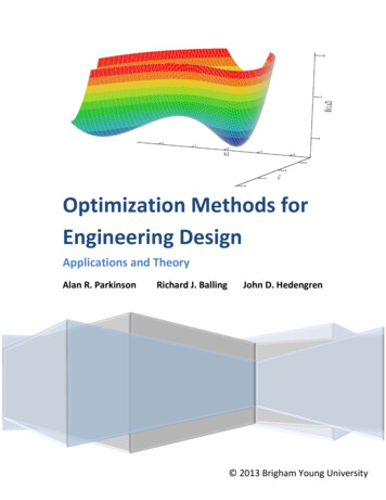
Chapter 1: Optimization Based DesignWe can easily see from the contours and the constraint boundaries that the optimum to thisproblem lies at the intersection of the buckling constraint and deflection constraint. We saythat these are binding (or active) constraints. Several other aspects of this optimum should benoted.First, this is a constrained optimum, since it lies on the constraint boundaries of buckling anddeflection. These constraints are binding or active. If we relaxed the allowable value forthese constraints, the optimum would improve. If we relaxed either of these constraintsenough, stress would become a binding constraint.It is possible to have an unconstrained optimum when we are optimizing, although not forthis problem. Assuming we are minimizing, the contours for such an optimum would looklike a valley. Contour plots showing unconstrained optimums are given in Fig. 1.10-3.001.003.00X1-AXISf ( x1 , x2 ) 4 4.5 x1 4 x2 x12 2 x22 2 x1 x2 x14 2 x12 x212-1.00

Chapter 1: Optimization-Based Designf ( x1 , x2 ) 4 4.5 x1 4 x2 x12 2 x22 2 x1 x2 x14 2 x12 x2Fig. 1.10 Contour plots which show unconstrained optimumsFig. 1.11. Surface plot of the function: 2242f x1 x2 4 4.5 x1 4 x2 x1 2 x2 2 x1 x2 x1 2 x1 x2.Second, this optimum is a local optimum. A local optimum is a point which has the bestobjective value of any feasible point in its neighborhood. We can see that no other near-byfeasible point has a better value than this optimum.Finally, this is also a global optimum. A global optimum is the best value over the entiredesign space. Obviously, a global optimum is also a local optimum. However, if we haveseveral local optimums, the global optimum is the best of these.13

Chapter 1: Optimization Based DesignIt is not always easy to tell whether we have a global optimum. Most optimization algorithmsonly guarantee finding a local optimum. In the example of the truss we can tell the optimumis global because, with only two variables, we can graph the entire space, and we can see thatthis is the only optimum in this space. If we have more than two variables, however, it isdifficult to graph the design space (and even if we could, it might be too expensive to do so)so we don’t always know for certain that a particular optimum is global. Often, to try todetermine if a particular solution is a global optimum, we start the optimization algorithmsfrom several different design points. If the algorithms always converge to the same spot, wehave some confidence that point is a global optimum.7. How Algorithms WorkThe most powerful optimization algorithms for nonlinear continuous problems usederivatives to determine a search direction in n dimensional space that improves theobjective and satisfies the constraints. Usually these derivatives are obtained numerically.For the Two-bar truss, search paths for two different starting points are given in Fig. 1.11Assuming derivatives are obtained numerically, the number of times the algorithms mustevaluate the model is roughly 10-15 times the number of optimization variables. Thus aproblem with 3 variables will require roughly 30-45 evaluations of the model; a problemwith 10 variables will require 100-150 model evaluations.StartingPoint 2StartingPoint 1Fig. 1.12. Two paths algorithms might follow for two different starting points.14

Chapter 1: Optimization-Based Design8. Cautions Regarding OptimizationOptimization algorithms can powerfully assist the designer in quantitative design synthesis.However,1. The designer should always carefully and thoroughly validate the engineering model.Optimization of an inaccurate model is modestly illuminating at best and misleading anda waste of time at worst. Often optimization algorithms will exploit weaknesses in themodel if they exist. As an example, regarding thermal systems, you can get some veryhigh performance designs if a model does not enforce the second law ofthermodynamics!2. The algorithms help a designer optimize a particular design concept. At no point will thealgorithms suggest that a different concept would be more appropriate. Achieving anoverall optimum is dependent upon selection of the best concept as well as quantitativeoptimization.3. Most engineering designs represent a compromise among conflicting objectives. Usuallythe designer will want to explore a number of alternative problem definitions to obtaininsight and understanding into the design space. Sometimes non-quantitativeconsiderations will drive the design in important ways.4. We need to make sure the optimization problem represents the real problem we need tosolve. Fox makes an important statement along these lines,“In engineering design we often feel that the objective functions are self evident. Butthere are pitfalls. Care must be taken to optimize with respect to the objectivefunction which most nearly reflects the true goals of the design problem. Someexamples of common errors.should help focus this point. In static structures, thefully utilized (fully stressed) design is not always the lightest weight; the lightestweight design is not always the cheapest; in mechanisms, the design with optimumtransmission angle does not necessarily have the lowest force levels; minimization ofacceleration level at the expense of jerk (third derivative) may result in inadequatedynamic response.”5. We need to be careful to optimize the system and not just individual parts. As anexample, the following poem by Oliver Wendell Holmes describes a “one horse” shay (awagon) so well built that it lasted 100 years, after which it went completely to pieces allat once.But the Deacon swore (as Deacons do),With an “I dew vum,” or an “I tell yeou,”He would build one shay to beat the taown‘N’ the keountry ‘n’ all the kentry raoun’;It should be so built that it couldn’ break daown:--”Fur,” said the Deacon, “‘t’s mighty plainThut the weakes’ place mus’ stan’ the strain;‘N’ the way t’ fix it, uz I maintain,Is only jest15

Chapter 1: Optimization Based DesignT’ make that place uz strong uz the rest.”.You see, of course, if you’re not a dunce,How it went to pieces all at once,-All at once, and nothing first,-Just as bubbles do when they burst.End of the wonderful one-hoss shay.Logic is logic. That’s all I say.Almost always in optimization we must take a system view, rather than an individualcomponent view.16

Chapter 2: Modeling ConceptsCHAPTER 2MODELING CONCEPTS1 IntroductionAs was discussed in the previous chapter, in order to apply optimization methods we musthave a model to optimize. As we also mentioned, obtaining a good model of the designproblem is the most important step in optimization. In this chapter we discuss some modelingconcepts that can help you develop models which can successfully be optimized. We alsodiscuss the formulation of objectives and constraints for some special situations. We look athow graphics can help us understand the nature of the design space and the model. We endwith an example optimization of a heat pump.2 Physical Models vs. Experimental ModelsTwo types of models are often used with optimization methods: physical models andexperimental models. Physical models are based on the underlying physical principles thatgovern the problem. Experimental models are based on models of experimental data. Somemodels contain both physical and experimental elements. We will discuss both types ofmodels briefly.2.1Physical ModelsPhysical models can be either analytical or numerical in nature. For example, the Two-bartruss is an analytical, physical model. The equations are based on modeling the physicalphenomena of stress, buckling stress and deflection. The equations are all closed form,analytical expressions. If we used numerical methods, such as the finite element method, tosolve for the solution to the model, we would have a numerical, physical model.2.2Experimental ModelsExperimental models are based on experimental data. A functional relationship for the data isproposed and fit to the data. If the fit is good, the model is retained; if not, a new relationshipis used. For example if we wish to find the friction factor for a pipe, we could refer to theMoody chart, or use expressions based on a curve fit of the data.3 Modeling Considerations3.1Making the Model RobustDuring optimization, the algorithms will move through the design space seeking an optimum.Sometime

A mechanical engineer designs a new engine, or a car suspension or a robot. A civil engineer designs a bridge or a building. A chemical engineer designs a distillation tower or a chemical process. An electrical engineer designs a computer or an integrated circuit.