Transcription
Practical Regression and Anova using RJulian J. FarawayJuly 2002
1Copyright c 1999, 2000, 2002 Julian J. FarawayPermission to reproduce individual copies of this book for personal use is granted. Multiple copies maybe created for nonprofit academic purposes — a nominal charge to cover the expense of reproduction maybe made. Reproduction for profit is prohibited without permission.
PrefaceThere are many books on regression and analysis of variance. These books expect different levels of preparedness and place different emphases on the material. This book is not introductory. It presumes someknowledge of basic statistical theory and practice. Students are expected to know the essentials of statisticalinference like estimation, hypothesis testing and confidence intervals. A basic knowledge of data analysis ispresumed. Some linear algebra and calculus is also required.The emphasis of this text is on the practice of regression and analysis of variance. The objective is tolearn what methods are available and more importantly, when they should be applied. Many examples arepresented to clarify the use of the techniques and to demonstrate what conclusions can be made. Thereis relatively less emphasis on mathematical theory, partly because some prior knowledge is assumed andpartly because the issues are better tackled elsewhere. Theory is important because it guides the approachwe take. I take a wider view of statistical theory. It is not just the formal theorems. Qualitative statisticalconcepts are just as important in Statistics because these enable us to actually do it rather than just talk aboutit. These qualitative principles are harder to learn because they are difficult to state precisely but they guidethe successful experienced Statistician.Data analysis cannot be learnt without actually doing it. This means using a statistical computing package. There is a wide choice of such packages. They are designed for different audiences and have differentstrengths and weaknesses. I have chosen to use R (ref. Ihaka and Gentleman (1996)). Why do I use R ?The are several reasons.1. Versatility. R is a also a programming language, so I am not limited by the procedures that arepreprogrammed by a package. It is relatively easy to program new methods in R .2. Interactivity. Data analysis is inherently interactive. Some older statistical packages were designedwhen computing was more expensive and batch processing of computations was the norm. Despiteimprovements in hardware, the old batch processing paradigm lives on in their use. R does one thingat a time, allowing us to make changes on the basis of what we see during the analysis.3. R is based on S from which the commercial package S-plus is derived. R itself is open-sourcesoftware and may be freely redistributed. Linux, Macintosh, Windows and other UNIX versionsare maintained and can be obtained from the R-project at www.r-project.org. R is mostlycompatible with S-plus meaning that S-plus could easily be used for the examples given in thisbook.4. Popularity. SAS is the most common statistics package in general but R or S is most popular withresearchers in Statistics. A look at common Statistical journals confirms this popularity. R is alsopopular for quantitative applications in Finance.The greatest disadvantage of R is that it is not so easy to learn. Some investment of effort is requiredbefore productivity gains will be realized. This book is not an introduction to R . There is a short introduction2
3in the Appendix but readers are referred to the R-project web site at www.r-project.org where youcan find introductory documentation and information about books on R . I have intentionally included inthe text all the commands used to produce the output seen in this book. This means that you can reproducethese analyses and experiment with changes and variations before fully understanding R . The reader maychoose to start working through this text before learning R and pick it up as you go.The web site for this book is at www.stat.lsa.umich.edu/ faraway/book where data described in this book appears. Updates will appear there also.Thanks to the builders of R without whom this book would not have been possible.
Contents123Introduction1.1 Before you start . . . . . . . . . .1.1.1 Formulation . . . . . . . .1.1.2 Data Collection . . . . . .1.1.3 Initial Data Analysis . . .1.2 When to use Regression Analysis .1.3 History . . . . . . . . . . . . . .Estimation2.1 Example . . . . . . . . . .2.2 Linear Model . . . . . . .2.3 Matrix Representation . .2.4 Estimating β . . . . . . . .2.5 Least squares estimation .2.6 Examples of calculating β̂2.7 Why is β̂ a good estimate?2.8 Gauss-Markov Theorem .2.9 Mean and Variance of β̂ . .2.10 Estimating σ2 . . . . . . .2.11 Goodness of Fit . . . . . .2.12 Example . . . . . . . . . .8. 8. 8. 9. 9. 13. 14.16161617171819192021212123Inference3.1 Hypothesis tests to compare models .3.2 Some Examples . . . . . . . . . . . .3.2.1 Test of all predictors . . . . .3.2.2 Testing just one predictor . . .3.2.3 Testing a pair of predictors . .3.2.4 Testing a subspace . . . . . .3.3 Concerns about Hypothesis Testing . .3.4 Confidence Intervals for β . . . . . .3.5 Confidence intervals for predictions .3.6 Orthogonality . . . . . . . . . . . . .3.7 Identifiability . . . . . . . . . . . . .3.8 Summary . . . . . . . . . . . . . . .3.9 What can go wrong? . . . . . . . . .3.9.1 Source and quality of the data.262628283031323336394144464646.4
CONTENTS53.9.2 Error component . . . . . . . . . . . . . . . . . . . . . . . . . . . . . . . . . . . . 473.9.3 Structural Component . . . . . . . . . . . . . . . . . . . . . . . . . . . . . . . . . 473.10 Interpreting Parameter Estimates . . . . . . . . . . . . . . . . . . . . . . . . . . . . . . . . 484Errors in Predictors555Generalized Least Squares5.1 The general case . . . . . . . . . . . . . . . . . . . . . . . . . . . . . . . . . . . . . . . .5.2 Weighted Least Squares . . . . . . . . . . . . . . . . . . . . . . . . . . . . . . . . . . . . .5.3 Iteratively Reweighted Least Squares . . . . . . . . . . . . . . . . . . . . . . . . . . . . . .595962646Testing for Lack of Fit656.1 σ2 known . . . . . . . . . . . . . . . . . . . . . . . . . . . . . . . . . . . . . . . . . . . . 666.2 σ2 unknown . . . . . . . . . . . . . . . . . . . . . . . . . . . . . . . . . . . . . . . . . . . 677Diagnostics7.1 Residuals and Leverage7.2 Studentized Residuals .7.3 An outlier test . . . . .7.4 Influential Observations7.5 Residual Plots . . . . .7.6 Non-Constant Variance7.7 Non-Linearity . . . . .7.8 Assessing Normality .7.9 Half-normal plots . . .7.10 Correlated Errors . . .89.7272747578808385889192Transformation8.1 Transforming the response . . .8.2 Transforming the predictors . . .8.2.1 Broken Stick Regression8.2.2 Polynomials . . . . . .8.3 Regression Splines . . . . . . .8.4 Modern Methods . . . . . . . 126128.Scale Changes, Principal Components and Collinearity9.1 Changes of Scale . . . . . . . . . . . . . . . . . . .9.2 Principal Components . . . . . . . . . . . . . . . . .9.3 Partial Least Squares . . . . . . . . . . . . . . . . .9.4 Collinearity . . . . . . . . . . . . . . . . . . . . . .9.5 Ridge Regression . . . . . . . . . . . . . . . . . . .10 Variable Selection10.1 Hierarchical Models . . . . .10.2 Stepwise Procedures . . . .10.2.1 Forward Selection .10.2.2 Stepwise Regression10.3 Criterion-based procedures .
CONTENTS610.4 Summary . . . . . . . . . . . . . . . . . . . . . . . . . . . . . . . . . . . . . . . . . . . . 13311 Statistical Strategy and Model Uncertainty13411.1 Strategy . . . . . . . . . . . . . . . . . . . . . . . . . . . . . . . . . . . . . . . . . . . . . 13411.2 Experiment . . . . . . . . . . . . . . . . . . . . . . . . . . . . . . . . . . . . . . . . . . . 13511.3 Discussion . . . . . . . . . . . . . . . . . . . . . . . . . . . . . . . . . . . . . . . . . . . . 13612 Chicago Insurance Redlining - a complete example13813 Robust and Resistant Regression15014 Missing Data15615 Analysis of Covariance16015.1 A two-level example . . . . . . . . . . . . . . . . . . . . . . . . . . . . . . . . . . . . . . 16115.2 Coding qualitative predictors . . . . . . . . . . . . . . . . . . . . . . . . . . . . . . . . . . 16415.3 A Three-level example . . . . . . . . . . . . . . . . . . . . . . . . . . . . . . . . . . . . . 16516 ANOVA16.1 One-Way Anova . . . . . . . . . . . . . . . . . . .16.1.1 The model . . . . . . . . . . . . . . . . .16.1.2 Estimation and testing . . . . . . . . . . .16.1.3 An example . . . . . . . . . . . . . . . . .16.1.4 Diagnostics . . . . . . . . . . . . . . . . .16.1.5 Multiple Comparisons . . . . . . . . . . .16.1.6 Contrasts . . . . . . . . . . . . . . . . . .16.1.7 Scheffé’s theorem for multiple comparisons16.1.8 Testing for homogeneity of variance . . . .16.2 Two-Way Anova . . . . . . . . . . . . . . . . . .16.2.1 One observation per cell . . . . . . . . . .16.2.2 More than one observation per cell . . . . .16.2.3 Interpreting the interaction effect . . . . . .16.2.4 Replication . . . . . . . . . . . . . . . . .16.3 Blocking designs . . . . . . . . . . . . . . . . . .16.3.1 Randomized Block design . . . . . . . . .16.3.2 Relative advantage of RCBD over CRD . .16.4 Latin Squares . . . . . . . . . . . . . . . . . . . .16.5 Balanced Incomplete Block design . . . . . . . . .16.6 Factorial experiments . . . . . . . . . . . . . . . 85190191195200A Recommended Books204A.1 Books on R . . . . . . . . . . . . . . . . . . . . . . . . . . . . . . . . . . . . . . . . . . . 204A.2 Books on Regression and Anova . . . . . . . . . . . . . . . . . . . . . . . . . . . . . . . . 204B R functions and data205
CONTENTSC Quick introduction to RC.1 Reading the data in . . . . .C.2 Numerical Summaries . . .C.3 Graphical Summaries . . . .C.4 Selecting subsets of the dataC.5 Learning more about R . . .7.207207207209209210
Chapter 1Introduction1.1 Before you startStatistics starts with a problem, continues with the collection of data, proceeds with the data analysis andfinishes with conclusions. It is a common mistake of inexperienced Statisticians to plunge into a complexanalysis without paying attention to what the objectives are or even whether the data are appropriate for theproposed analysis. Look before you leap!1.1.1 FormulationThe formulation of a problem is often more essential than its solution which may be merely amatter of mathematical or experimental skill. Albert EinsteinTo formulate the problem correctly, you must1. Understand the physical background. Statisticians often work in collaboration with others and needto understand something about the subject area. Regard this as an opportunity to learn something newrather than a chore.2. Understand the objective. Again, often you will be working with a collaborator who may not be clearabout what the objectives are. Beware of “fishing expeditions” - if you look hard enough, you’llalmost always find something but that something may just be a coincidence.3. Make sure you know what the client wants. Sometimes Statisticians perform an analysis far morecomplicated than the client really needed. You may find that simple descriptive statistics are all thatare needed.4. Put the problem into statistical terms. This is a challenging step and where irreparable errors aresometimes made. Once the problem is translated into the language of Statistics, the solution is oftenroutine. Difficulties with this step explain why Artificial Intelligence techniques have yet to makemuch impact in application to Statistics. Defining the problem is hard to program.That a statistical method can read in and process the data is not enough. The results may be totallymeaningless.8
1.1. BEFORE YOU START91.1.2 Data CollectionIt’s important to understand how the data was collected.Are the data observational or experimental? Are the data a sample of convenience or were theyobtained via a designed sample survey. How the data were collected has a crucial impact on whatconclusions can be made.Is there non-response? The data you don’t see may be just as important as the data you do see.Are there missing values? This is a common problem that is troublesome and time consuming to dealwith.How are the data coded? In particular, how are the qualitative variables represented.What are the units of measurement? Sometimes data is collected or represented with far more digitsthan are necessary. Consider rounding if this will help with the interpretation or storage costs.Beware of data entry errors. This problem is all too common — almost a certainty in any real datasetof at least moderate size. Perform some data sanity checks.1.1.3 Initial Data AnalysisThis is a critical step that should always be performed. It looks simple but it is vital.Numerical summaries - means, sds, five-number summaries, correlations.Graphical summaries– One variable - Boxplots, histograms etc.– Two variables - scatterplots.– Many variables - interactive graphics.Look for outliers, data-entry errors and skewed or unusual distributions. Are the data distributed as youexpect?Getting data into a form suitable for analysis by cleaning out mistakes and aberrations is often timeconsuming. It often takes more time than the data analysis itself. In this course, all the data will be ready toanalyze but you should realize that in practice this is rarely the case.Let’s look at an example. The National Institute of Diabetes and Digestive and Kidney Diseasesconducted a study on 768 adult female Pima Indians living near Phoenix. The following variables wererecorded: Number of times pregnant, Plasma glucose concentration a 2 hours in an oral glucose tolerancetest, Diastolic blood pressure (mm Hg), Triceps skin fold thickness (mm), 2-Hour serum insulin (mu U/ml),Body mass index (weight in kg/(height in m 2 )), Diabetes pedigree function, Age (years) and a test whetherthe patient shows signs of diabetes (coded 0 if negative, 1 if positive). The data may be obtained from UCIRepository of machine learning databases at http://www.ics.uci.edu/ mlearn/MLRepository.html.Of course, before doing anything else, one should find out what the purpose of the study was and moreabout how the data was collected. But let’s skip ahead to a look at the data:
1.1. BEFORE YOU START10 library(faraway) data(pima) pimapregnant glucose diastolic triceps insulin bmi diabetes age test1614872350 33.60.627 501218566290 26.60.351 310381836400 23.30.672 321. much deleted .76819370310 30.40.315 230The library(faraway) makes the data used in this book available while data(pima) calls upthis particular dataset. Simply typing the name of the data frame, pima prints out the data. It’s too long toshow it all here. For a dataset of this size, one can just about visually skim over the data for anything out ofplace but it is certainly easier to use more direct methods.We start with some numerical summaries: summary(pima)pregnantMin.: 0.001st Qu.: 1.00Median : 3.00Mean: 3.853rd Qu.: 6.00Max.:17.00bmiMin.: 0.01st Qu.:27.3Median :32.0Mean:32.03rd Qu.:36.6Max.:67.1glucoseMin.: 01st Qu.: 99Median :117Mean:1213rd Qu.:140Max.:199diabetesMin.:0.0781st Qu.:0.244Median :0.372Mean:0.4723rd Qu.:0.626Max.:2.420diastolicMin.: 0.01st Qu.: 62.0Median : 72.0Mean: 69.13rd Qu.: 80.0Max.:122.0ageMin.:21.01st Qu.:24.0Median :29.0Mean:33.23rd Qu.:41.0Max.:81.0tricepsMin.: 0.01st Qu.: 0.0Median :23.0Mean:20.53rd Qu.:32.0Max.:99.0testMin.:0.0001st Qu.:0.000Median :0.000Mean:0.3493rd Qu.:1.000Max.:1.000insulinMin.: 0.01st Qu.: 0.0Median : 30.5Mean: 79.83rd Qu.:127.2Max.:846.0The summary() command is a quick way to get the usual univariate summary information. At this stage,we are looking for anything unusual or unexpected perhaps indicating a data entry error. For this purpose, aclose look at the minimum and maximum values of each variable is worthwhile. Starting with pregnant,we see a maximum value of 17. This is large but perhaps not impossible. However, we then see that the next5 variables have minimum values of zero. No blood pressure is not good for the health — something mustbe wrong. Let’s look at the sorted values: sort(pima diastolic)[1]00000[19]00000[37] 30 30 38 40 00050We see that the first 36 values are zero. The description that comes with the data says nothing about it butit seems likely that the zero has been used as a missing value code. For one reason or another, the researchersdid not obtain the blood pressures of 36 patients. In a real investigation, one would likely be able to questionthe researchers about what really happened. Nevertheless, this does illustrate the kind of misunderstanding02450
1.1. BEFORE YOU START11that can easily occur. A careless statistician might overlook these presumed missing values and complete ananalysis assuming that these were real observed zeroes. If the error was later discovered, they might thenblame the researchers for using 0 as a missing value code (not a good choice since it is a valid value forsome of the variables) and not mentioning it in their data description. Unfortunately such oversights arenot uncommon particularly with datasets of any size or complexity. The statistician bears some share ofresponsibility for spotting these mistakes.We set all zero values of the five variables to NA which is the missing value code used by R . pima diastolic[pima diastolic 0] - NApima glucose[pima glucose 0] - NApima triceps[pima triceps 0] - NApima insulin[pima insulin 0] - NApima bmi[pima bmi 0] - NAThe variable test is not quantitative but categorical. Such variables are also called factors. However,because of the numerical coding, this variable has been treated as if it were quantitative. It’s best to designatesuch variables as factors so that they are treated appropriately. Sometimes people forget this and computestupid statistics such as “average zip code”. pima test - factor(pima test) summary(pima test)01500 268We now see that 500 cases were negative and 268 positive. Even better is to use descriptive labels: levels(pima test) - c("negative","positive") summary(pima)pregnantglucosediastolictricepsMin.: 0.00Min.: 44Min.: 24.0Min.: 7.01st Qu.: 1.001st Qu.: 991st Qu.: 64.01st Qu.: 22.0Median : 3.00Median :117Median : 72.0Median : 29.0Mean: 3.85Mean:122Mean: 72.4Mean: 29.23rd Qu.: 6.003rd Qu.:1413rd Qu.: 80.03rd Qu.: 36.0Max.:17.00Max.:199Max.:122.0Max.: 99.0NA’s: 5NA’s: 078Min.:21.0negative:5001st Qu.:27.51st Qu.:0.2441st Qu.:24.0positive:268Median :32.3Median :0.372Median :29.0Mean:32.5Mean:0.472Mean:33.23rd Qu.:36.63rd Qu.:0.6263rd ulinMin.: 14.01st Qu.: 76.2Median :125.0Mean:155.53rd Qu.:190.0Max.:846.0NA’s:374.0Now that we’ve cleared up the missing values and coded the data appropriately we are ready to do someplots. Perhaps the most well-known univariate plot is the histogram:hist(pima diastolic)
1.1. BEFORE YOU START0sort(pima cy1001502000.0301201220406080 100 120pima diastolic20 40 60 80 100 120N 733 Bandwidth 2.8720200400Index600Figure 1.1: First panel shows histogram of the diastolic blood pressures, the second shows a kernel densityestimate of the same while the the third shows an index plot of the sorted valuesas shown in the first panel of Figure 1.1. We see a bell-shaped distribution for the diastolic blood pressurescentered around 70. The construction of a histogram requires the specification of the number of bins andtheir spacing on the horizontal axis. Some choices can lead to histograms that obscure some features of thedata. R attempts to specify the number and spacing of bins given the size and distribution of the data butthis choice is not foolproof and misleading histograms are possible. For this reason, I prefer to use KernelDensity Estimates which are essentially a smoothed version of the histogram (see Simonoff (1996) for adiscussion of the relative merits of histograms and kernel estimates). plot(density(pima diastolic,na.rm TRUE))The kernel estimate may be seen in the second panel of Figure 1.1. We see that it avoids the distractingblockiness of the histogram. An alternative is to simply plot the sorted data against its index:plot(sort(pima diastolic),pch ".")The advantage of this is we can see all the data points themselves. We can see the distribution andpossible outliers. We can also see the discreteness in the measurement of blood pressure - values are roundedto the nearest even number and hence we the “steps” in the plot.Now a couple of bivariate plots as seen in Figure 1.2: plot(diabetes diastolic,pima) plot(diabetes test,pima)hist(pima diastolic)First, we see the standard scatterplot showing two quantitative variables. Second, we see a side-by-sideboxplot suitable for showing a quantitative and a qualititative variable. Also useful is a scatterplot matrix,not shown here, produced by
2.02.5130.00.5diabetes1.0 1.50.00.5diabetes1.0 1.52.02.51.2. WHEN TO USE REGRESSION igure 1.2: First panel shows scatterplot of the diastolic blood pressures against diabetes function and thesecond shows boxplots of diastolic blood pressure broken down by test result pairs(pima)We will be seeing more advanced plots later but the numerical and graphical summaries presented here aresufficient for a first look at the data.1.2 When to use Regression AnalysisRegression analysis is used for explaining or modeling the relationship between a single variable Y , calledthe response, output or dependent variable, and one or more predictor, input, independent or explanatory variables, X1 X p . When p 1, it is called simple regression but when p 1 it is called multiple regression or sometimes multivariate regression. When there is more than one Y , then it is called multivariatemultiple regression which we won’t be covering here.The response must be a continuous variable but the explanatory variables can be continuous, discreteor categorical although we leave the handling of categorical explanatory variables to later in the course.Taking the example presented above, a regression of diastolic and bmi on diabetes would be amultiple regression involving only quantitative variables which we shall be tackling shortly. A regression ofdiastolic and bmi on test would involve one predictor which is quantitative which we will considerin later in the chapter on Analysis of Covariance. A regression of diastolic on just test would involvejust qualitative predictors, a topic called Analysis of Variance or ANOVA although this would just be a simpletwo sample situation. A regression of test (the response) on diastolic and bmi (the predictors) wouldinvolve a qualitative response. A logistic regression could be used but this will not be covered in this book.Regression analyses have several possible objectives including1. Prediction of future observations.2. Assessment of the effect of, or relationship between, explanatory variables on the response.3. A general description of data structure.
1.3. HISTORY14Extensions exist to handle multivariate responses, binary responses (logistic regression analysis) andcount responses (poisson regression).1.3 HistoryRegression-type problems were first considered in the 18th century concerning navigation using astronomy.Legendre developed the method of least squares in 1805. Gauss claimed to have developed the method afew years earlier and showed that the least squares was the optimal solution when the errors are normallydistributed in 1809. The methodology was used almost exclusively in the physical sciences until later in the19th century. Francis Galton coined the term regression to mediocrity in 1875 in reference to the simpleregression equation in the formx x̄y ȳ r SDySDx Galton used this equation to explain the phenomenon that sons of tall fathers tend to be tall but not as tall astheir fathers while sons of short fathers tend to be short but not as short as their fathers. This effect is calledthe regression effect.We can illustrate this effect with some data on scores from a course taught using this book. In Figure 1.3,we see a plot of midterm against final scores. We scale each variable to have mean 0 and SD 1 so that we arenot distracted by the relative difficulty of each exam and the total number of points possible. Furthermore,this simplifies the regression equation toy rxdata(stat500)stat500 - data.frame(scale(stat500))plot(final midterm,stat500)abline(0,1) 2final 1012 2 10midterm12Figure 1.3: Final and midterm scores in standard units. Least squares fit is shown with a dotted line whiley x is shown as a solid line
1.3. HISTORY15We have added the y x (solid) line to the plot. Now a student scoring, say one standard deviationabove average on the midterm might reasonably expect to do equally well on the final. We compute theleast squares regression fit and plot the regression line (more on the details later). We also compute thecorrelations. g - lm(final midterm,stat500) abline(g coef,lty 5) cor(stat500)midtermfinalhwtotalmidterm 1.00000 0.545228 0.272058 0.84446final0.54523 1.000000 0.087338 0.77886hw0.27206 0.087338 1.000000 0.56443total0.84446 0.778863 0.564429 1.00000We see that the the student scoring 1 SD above average on the midterm is predicted to score somewhatless above average on the final (see the dotted regression line) - 0.54523 SD’s above average to be exact.Correspondingly, a student scoring below average on the midterm might expect to do relatively better in thefinal although still below average.If exams managed to measure the ability of students perfectly, then provided that ability remained unchanged from midterm to final, we would expect to see a perfect correlation. Of course, it’s too much toexpect such a perfect exam and some variation is inevitably present. Furthermore, individual effort is notconstant. Getting a high score on the midterm can partly be attributed to skill but also a certain amount ofluck. One cannot rely on this luck to be maintained in the final. Hence we see the “regression to mediocrity”.Of course this applies to any x y situation like this — an example is the so-called sophomore jinxin sports when a rookie star has a so-so second season after a great first year. Although in the father-sonexample, it does predict that successive descendants will come closer to the mean, it does not imply thesame of the population in general since random fluctuations will maintain the variation. In many otherapplications of regression, the regression effect is not of interest so it is unfortunate that we are now stuckwith this rather misleading name.Regression methodology developed rapidly with the advent of high-speed computing. Just fitting aregression model used to require extensive hand calculation. As computing hardware has improved, thenthe scope for analysis has widened.
Chapter 2Estimation2.1 ExampleLet’s start with an example. Suppose that Y is the fuel consumption of a particular model of car in m.p.g.Suppose that the predictors are1. X1 — the weight of the car2. X2 — the horse power3. X3 — the no. of cylinders.X3 is discrete but that’s OK. Using country of origin, say, as a predictor would not be possible within thecurrent develop
book. 4. Popularity. SAS is the most common statistics package in general but R or S is most popular with researchers in Statistics. A look at common Statistical journals confirms this popularity. R is also popular for quantitative applications in Finance. The greatest disadvantage of R is that it is not so easy to learn.