Transcription
Barrier Option PricingDegree Project in Mathematics, First LevelNiklas WestermarkAbstractThis thesis examines the performance of five option pricing models with respect to the pricing ofbarrier options. The models include the Black-Scholes model and four stochastic volatilitymodels ranging from the single-factor stochastic volatility model first proposed by Heston (1993)to a multi-factor stochastic volatility model with jumps in the spot price process. The stochasticvolatility models are calibrated using four different loss functions to examine the loss functionseffect on the resulting barrier option prices. Our results show that the Black-Scholes model yieldssignificantly different prices than the stochastic volatility models for barriers far from the currentspot price. The prices of the four stochastic volatility models are however very similar. We alsoshow that the choice of loss function for parameter estimation has little effect on the obtainedbarrier option prices.Acknowledgements:I would like to thank my tutor Camilla Landén for helpful advice during the writing of this thesis.
Table of contents1.Introduction . 11.1.2.3.4.5.6.Barrier options . 1Model presentation . 22.1.Stochastic volatility model (SV). 32.2.Stochastic volatility model with jumps (SVJ) . 32.3.Multi-factor stochastic volatility model (MFSV) . 42.4.Multi-factor stochastic volatility model with jumps (MFSVJ) . 5Vanilla option pricing. 63.1.Option pricing in the Black-Scholes model . 63.2.Option pricing in stochastic volatility models . 6Parameter estimation . 84.1.Data . 94.2.Loss function . 94.3.Estimation procedure . 12Barrier option pricing . 125.1.Black-Scholes model . 125.2.Monte Carlo simulation . 135.2.1.SV model . 145.2.2.SVJ model . 145.2.3.MFSV model . 145.2.4.MFSVJ model . 15Results . 156.1.Parameter estimates and in-sample fit . 156.2.Barrier option prices . 167.Conclusion . 188.References . 19Appendix A: Tables and graphs . 21Appendix B: Data . 36i
1.IntroductionEver since the presentation of the famous Black & Scholes model [7], academics andpractitioners have made numerous attempts to relax the restrictive assumptions that make themodel inconsistent with observed prices in the market. Particular interest has been directedtowards the assumption of constant volatility, which makes the model unable to generate nonnormal return distributions and the well-known volatility smile, consistent with empiricalfindings on asset returns [12].Examples of extensions of the Black-Scholes model include models that allow for stochasticvolatility and jumps in the underlying return process. Many different models have been proposed,ranging from single-factor stochastic volatility models, to multi-factor models with log-normallydistributed jumps in the stock price process as well as stochastic interest rates (see e.g. [3], [4],[5], [11], [19] and [27]).In a recognized paper, Schoutens, Simons & Tistaert [23] show that although there are manyoption pricing models available that very accurately can explain observed prices of plain vanillaoptions, the models may produce inconsistent prices when applied to more exotic derivatives. Inthis thesis, we extend the results of [23] by conducting a similar analysis with four stochasticvolatility models, including two multi-factor stochastic volatility models not examined in [23].All four models allow for non-normal return distributions and non-constant volatility and haveproven to be effective in the pricing of plain vanilla call and put options (see e.g. [3], [5] and[23]). We also extend the estimation technique by calibrating the models using four different lossfunctions, and examine how the choice of loss function potentially affects the pricingperformance of the models.To estimate the model parameters, we use the same data set as in [23], i.e. the implied volatilitysurface of the Eurostoxx 50 index on the 7th of October 2003. Using the estimated modelparameters, we analyze the models’ pricing performance with respect to the commonly tradedexotic options called barrier options, and compare the obtained prices using the different modelsand loss functions.Our results show that the prices of barrier options differ significantly between the Black-Scholesmodel and the stochastic volatility models. We also show that the choice of loss function forestimation of model parameters in the stochastic volatility models have little effect on theresulting barrier option prices.1.1. Barrier optionsA barrier option is a path-dependent option whose pay-off at maturity depends on whether or notthe underlying spot price has touched some pre-defined barrier during the life of the option. Inthis thesis, we will limit our attention to four of the most common barrier options, namely upand-in (UI), up-and-out (UO), down-and-in (DI) and down-and-out (DO) call options.1
To describe the pay-off structures of the barrier options, define the maximum and the minimumof the spot price process 𝑆 𝑆𝑡 , 0 𝑡 𝑇 as 𝑚𝑆 inf 𝑆𝑡 ; 0 𝑡 𝑇 and 𝑀𝑆 sup 𝑆𝑡 ; 0 𝑡 𝑇 .The UI call option is worthless unless the underlying spot price 𝑆 hits a pre-determined barrier𝐻 𝑆0 during the life of the option, in which case it becomes a standard call option. Hence, itspay-off at maturity is:Φ𝑈𝐼 𝑆𝑇 , 𝑀𝑆 𝑆𝑇 𝐾 𝟏(𝑀𝑆 𝐻)(1.1)where 𝟏(𝑀𝑆 𝐻) is an indicator function equal to one if 𝑀𝑆 𝐻 and zero otherwise.For the UO call option, the relationship is reversed: the UO call option is a standard call optionunless the underlying spot price hits the barrier, in which case it becomes worthless:Φ𝑈𝑂 𝑆𝑇 , 𝑚𝑆 𝑆𝑇 𝐾 𝟏(𝑚𝑆 𝐻)(1.2)For DI and DO call options, the barrier 𝐻 is set below the spot price at inception, 𝐻 𝑆0 . Thepay-off structures of the DI and DO options follow analogously: the DI call option is worthlessunless the barrier 𝐻 is reached some time during the life of the trade, in which case it becomes aplain vanilla call option. The DO option, on the other hand, is a standard call option unless thespot price reaches the lower barrier during the life of the option, in which case it becomesworthless. The pay-off structures of the DI and DO call options are:2.Φ𝐷𝐼 𝑆𝑇 , 𝑚𝑆 𝑆𝑇 𝐾 Φ𝐷𝑂 𝑆𝑇 , 𝑀𝑆 𝑆𝑇 𝐾 𝟏(𝑚𝑆 𝐻)𝟏(𝑀𝑆 𝐻)(1.3)(1.4)Model presentationWe will assume that the reader has a basic knowledge of the basic Black-Scholes framework andwill thus refrain from describing the Black-Scholes model in detail. The interested reader isreferred to [21] for an economic outline and to [6] for a description of the mathematicalframework.For all models, we consider the risk-neutral dynamics of the stock price. We let 𝑆 𝑆𝑡 , 0 𝑡 𝑇 denote the stock price process and 𝜑 𝑇 ( ) denote the characteristic function of thenatural logarithm of the terminal stock price 𝑠𝑇 log 𝑆𝑇 , where log denotes the naturallogarithm function. The constants 𝑟 and 𝛿 will denote the, both constant and continuouslycompounded, interest rate and dividend yield, respectively. Further, we let 𝑊𝑡ℚ denote a ℚWiener process.2
2.1. Stochastic volatility model (SV)Many different stochastic volatility models have been proposed, but we will limit our attention tothe Heston [19] stochastic volatility model, henceforth denoted SV, in which the spot price isdescribed by the following stochastic differential equations (SDEs) under ℚ:𝑑𝑆𝑡ℚ (1) 𝑟 𝛿 𝑑𝑡 𝑉𝑡 𝑑𝑊𝑡𝑆𝑡𝑑𝑉𝑡 𝜅 𝜃 𝑉𝑡 𝑑𝑡 𝜍 𝑉𝑡 𝑑𝑊𝑡ℚ 2𝑑𝑊𝑡ℚ1𝑑𝑊𝑡ℚ2 𝜌𝑑𝑡(2.1)(2.2)(2.3)where 𝑉𝑡 is the stochastic variance and the parameters 𝜅, 𝜃, 𝜍 and 𝜌 represent the speed of meanreversion, the long-run mean of the variance, the volatility of the variance process and thecorrelation between the variance and stock price processes, respectively. In addition to theseparameters, the model requires the estimation of the instantaneous spot variance 𝑉0 .Using the same representation of the parameters as in equations (2.1) – (2.3), the characteristicfunction of 𝑠𝑇 takes the following form:𝜑𝑇𝑆𝑉 𝑢 𝑆0𝑖𝑢 𝑓(𝑉0 , 𝑢, 𝑇)(2.4)where𝑓 𝑉0 , 𝑢, 𝑇 exp 𝐴 𝑢, 𝑇 𝐵 𝑢, 𝑇 𝑉0𝜅𝜃1 𝑔𝑒 𝑑𝑇𝐴 𝑢, 𝑇 𝑟 𝛿 𝑖𝑢𝑇 2 (𝜅 𝜌𝜍𝑖𝑢 𝑑)𝑇 2 log𝜍1 𝑔𝜅 𝜌𝜍𝑖𝑢 𝑑 1 𝑒 𝑑𝑇𝐵 𝑢, 𝑇 𝜍21 𝑔𝑒 𝑑𝑇𝑑 𝜌𝜍𝑖𝑢 𝜅 2 𝜍 2 (𝑖𝑢 𝑢2 )𝑔 (𝜅 𝜌𝜍𝑖𝑢 𝑑)/(𝜅 𝜌𝜍𝑖𝑢 𝑑)(2.5)(2.6)(2.7)(2.8)(2.9)2.2. Stochastic volatility model with jumps (SVJ)We extend the SV model in the previous section along the lines of [4], by adding log-normallydistributed jumps to the stock price process. In this model, here denoted SVJ, the return processof the spot price is described by the following set of SDEs under ℚ:𝑑𝑆𝑡ℚ (1) 𝑟 𝛿 𝜆𝜇𝐽 𝑑𝑡 𝑉𝑡 𝑑𝑊𝑡 𝐽𝑡 𝑑𝑌𝑡𝑆𝑡𝑑𝑉𝑡 𝜅 𝜃 𝑉𝑡 𝑑𝑡 𝜍 𝑉𝑡 𝑑𝑊𝑡ℚ 2𝑑𝑊𝑡ℚ 1𝑑𝑊𝑡ℚ 2 𝜌𝑑𝑡(2.10)(2.11)(2.12)where 𝑌 𝑌𝑡 , 0 𝑡 𝑇 is a Poisson process with intensity 𝜆 0 and 𝐽𝑡 is the jump sizeconditional on a jump occurring. All other parameters are defined as in (2.1) – (2.3). Thesubtraction of 𝜆𝜇𝐽 in the drift term compensates for the expected drift added by the jump3
component, so that the total drift of the process, as required for risk-neutral valuation, remains(𝑟 𝑞)𝑑𝑡.As mentioned, the jump size is assumed to be log-normally distributed:log 1 𝐽𝑡 𝑁 log 1 𝜇𝐽 𝜍𝐽2 2,𝜍2 𝐽(2.13)ℚ (1)Further, it is assumed that 𝑌𝑡 and 𝐽𝑡 are independent of each other as well as of 𝑊𝑡ℚ (2)and 𝑊𝑡.Using the independence of 𝑌𝑡 , 𝐽𝑡 and the two Wiener processes, one can show that thecharacteristic function of the SVJ model is [15]:𝑆𝑉𝐽𝐽𝜑𝑇 (𝑢) 𝜑𝑇𝑆𝑉 (𝑢) 𝜑𝑇 (𝑢)(2.14)𝜑𝑇𝐽 exp{ 𝜆𝜇𝐽 𝑖𝑢𝑇 𝜆𝑇((1 𝜇𝐽 ) 𝑖𝑢 exp(𝜍𝐽2 (𝑖𝑢/2)(𝑖𝑢 1)) 1)}(2.15)where:and 𝜑 𝑇𝑆𝑉 (𝑢) is defined as in (2.4).2.3. Multi-factor stochastic volatility model (MFSV)The multi-factor stochastic volatility model is an extension of the SV model and has been studiedby e.g. [5] and [10]. We denote the multi-factor stochastic volatility model MFSV and let thefollowing set of SDEs describe the return process under the risk-neutral measure:𝑑𝑆𝑡(1)ℚ (1)(2)ℚ (2) 𝑟 𝛿 𝑑𝑡 𝑉𝑡 𝑑𝑊𝑡 𝑉𝑡 𝑑𝑊𝑡𝑆𝑡𝑑𝑉𝑡1 𝜅1 𝜃1 𝑉𝑡1𝑑𝑡 𝜍1 𝑉𝑡1𝑑𝑊𝑡𝑑𝑉𝑡2 𝜅2 𝜃2 𝑉𝑡2𝑑𝑡 𝜍2 𝑉𝑡2𝑑𝑊𝑡(2.16)ℚ 3(2.17)ℚ 4(2.18)where the parameters have the same meaning as in (2.1) – (2.3) and the subscripts 1 and 2indicate to which variance process the parameter is related.The dependence structure is assumed to be as follows:ℚ 𝑖𝑑𝑊𝑡ℚ𝑑𝑊𝑡𝑑𝑊𝑡ℚ 1 𝑑𝑊𝑡ℚ 3 𝜌1 𝑑𝑡𝑑𝑊𝑡ℚ 2 𝑑𝑊𝑡ℚ 4 𝜌2 𝑑𝑡𝑗 0,𝑖, 𝑗 1,2 , 1,4 , 2,3 , (3,4)4(2.19)(2.20)(2.21)
In other words, each variance process is correlated with the corresponding Wiener process in thereturn process, i.e. the diffusion term of which the respective variance process determines themagnitude.By the independence structure described above, the added diffusion term is independent of thenested SV model return SDE. Since the characteristic function of the sum of two independentvariables is the product of their individual characteristic functions, the characteristic function ofthe MFSV model is determined as:𝑖𝑢 𝑠𝑇𝜑𝑀𝐹𝑆𝑉(𝑢) 𝔼ℚ 𝑆0𝑖𝑢 𝑓 𝑉0 1 , 𝑉0 2 , 𝑢, 𝑇𝑇0 𝑒(2.22)where:12𝑓 𝑉0 , 𝑉0 , 𝑢, 𝑇 exp 𝐴 𝑢, 𝑇 𝐵1 𝑢, 𝑇 𝑉0𝐴 𝑢, 𝑇 𝑟 𝛿 𝑖𝑢𝑇 2𝑗 1𝜍𝑗 2 𝜅𝑗 𝜃𝑗𝑑𝑗 𝐵2 𝑢, 𝑇 𝑉0𝜅𝑗 𝜌𝑗 𝜍𝑗 𝑖𝑢 𝑑𝑗 𝑇 2 log𝐵𝑗 𝑢, 𝑇 𝜍𝑗 2 (𝜅𝑗 𝜌𝑗 𝜍𝑗 𝑖𝑢 𝑑𝑗 )𝑔𝑗 1𝜅𝑗 𝜌𝑗 𝜍𝑗 𝑖𝑢 𝑑𝑗𝜅𝑗 𝜌𝑗 𝜍𝑗 𝑖𝑢 𝑑𝑗𝜌𝑗 𝜍𝑗 𝑖𝑢 𝜅𝑗21 𝑒 𝑑 𝑗 𝑇21 𝑔𝑗 𝑒 𝑑 𝑗 𝑇1 𝑔𝑗(2.23)(2.24)(2.25)1 𝑔𝑗 𝑒 𝑑 𝑗 𝑇(2.26) 𝜍 𝑗2 (𝑖𝑢 𝑢2 )(2.27)2.4. Multi-factor stochastic volatility model with jumps (MFSVJ)The multi-factor stochastic volatility model with jumps that we use in this paper is a variation ofthe model presented in [5]. However, we use a different approach in the sense that we estimatethe model to only one day’s data whereas [5] uses a data set spanning over 7 years. We denotethe multi-factor stochastic volatility model with jumps MFSVJ, and let the risk-neutral stockprice dynamics be described by the following set of SDEs:𝑑𝑆𝑡(1)ℚ (1)(2)ℚ (2) 𝑟 𝛿 𝜆𝜇𝐽 𝑑𝑡 𝑉𝑡 𝑑𝑊𝑡 𝑉𝑡 𝑑𝑊𝑡 𝐽𝑡 𝑑𝑌𝑡𝑆𝑡(2.28)𝑑𝑉𝑡1 𝜅1 𝜃1 𝑉𝑡1𝑑𝑡 𝜍1 𝑉𝑡1𝑑𝑊𝑡ℚ3(2.29)𝑑𝑉𝑡1 𝜅2 𝜃2 𝑉𝑡2𝑑𝑡 𝜍2 𝑉𝑡2𝑑𝑊𝑡ℚ4(2.30)where all parameters and variables are defined as in equations (2.1) – (2.3) and (2.10). Thedistributions of 𝐽𝑡 and 𝑌𝑡 are log-normal and Poisson, respectively, according to equations (2.10)and (2.13), and the two variables are independent, both of each other and of the four Wienerprocesses. The dependence structure between the Wiener processes is the same as in the MFSVmodel according to equations (2.19) – (2.21).5
Due to the independence between the added jump factor and the SDE of the MFSV model, thecharacteristic function of 𝑠𝑇 is obtained in the same way as in the SVJ model, i.e. as the productof the jump-term characteristic function and the characteristic function of the MFSV model:𝜑𝑇𝑀𝐹𝑆𝑉𝐽 (𝑢) 𝜑𝑀𝐹𝑆𝑉(𝑢) 𝜑𝑇𝐽 (𝑢)𝑇(2.31)where 𝜑 𝑀𝐹𝑆𝑉(𝑢) and 𝜑𝑇𝐽 𝑢 are defined in equations (2.22) and (2.15), respectively.𝑇3.Vanilla option pricing3.1. Option pricing in the Black-Scholes modelOne of the most appealing features of the Black-Scholes model is the existence of an analyticalformula for the pricing of European call and put options. Given that the model parameters(essentially 𝜍) are known, the Black-Scholes price of a European call or put option is calculatedas:𝑃𝑟𝑖𝑐𝑒𝑡𝐵𝑆 𝑆𝑡 𝑒 𝛿(𝑇 𝑡) 𝑁 𝜔𝑑1 𝜔𝐾𝑒 𝑟(𝑇 𝑡) 𝑁 𝜔𝑑2(3.1)where 𝑆𝑡 denotes the spot price, 𝐾 the strike price, 𝑟 the interest rate, 𝑞 the dividend yield, 𝑇 𝑡the time to maturity and 𝜔 is a binary operator equal to 1 for call options and 1 for put options.Further, we have that:𝑑1 log𝑆𝑡𝜍2 𝑟 𝛿 𝐾2𝜍 𝑇 𝑡𝑑2 𝑑1 𝜍 𝑇 𝑡𝑇 𝑡(3.2)(3.3)in which 𝜍 is the volatility of the spot price.3.2. Option pricing in stochastic volatility modelsAssuming that the characteristic function of the log-stock price is known analytically, the price ofplain vanilla options can be determined using the Fast Fourier Transform (FFT) method firstpresented in [8]. Using this approach, the call price is expressed in terms of an inverse Fouriertransform of the characteristic function of the log-stock price under the assumed stochasticprocess. The resulting formula can then be re-formulated to enable computation using the FFTalgorithm that significantly decreases computation time compared to standard numerical methodssuch as the discrete Fourier transform.To derive the call price function in the FFT approach, we follow closely the method of [8], whilealso allowing for a continuous dividend yield 𝛿 . Denote by 𝑠𝑇 and 𝑘 the natural logarithm ofthe terminal stock price and the strike price 𝐾, respectively. Further, let 𝐶𝑇 𝑘 denote the value ofa European call option with pay-off function 𝑓 𝑆𝑇 𝑆𝑇 𝐾 𝑒 𝑠𝑇 𝑒 𝑘 and maturity attime 𝑇. The discounted expected pay-off under ℚ is then:6
𝐶𝑇 𝑘 𝔼ℚ𝑡𝑒 𝑟𝑇 𝑆𝑇 𝐾𝑒 𝑟𝑇 𝑒 𝑠𝑇 𝑒 𝑘 𝑞𝑇 𝑠𝑇 𝑑𝑠𝑇 (3.4)𝑘where 𝑞𝑇 (𝑠) is the risk-neutral density of 𝑠𝑇 . As 𝑘 tends to , (3.4) translates to: 𝑒 𝑟𝑇 𝑒 𝑠𝑇 𝑞𝑇 𝑠𝑇 𝑑𝑠𝑇 𝑒 𝑟𝑇 𝔼ℚ𝑡 𝑆𝑇 𝑆0lim 𝐶𝑇 𝑘 k (3.5) This is on the one hand reassuring, as the price of a call with a strike price of zero shouldequal 𝑆0 . On the other hand, in order to apply the Fourier transform to 𝐶𝑇 (𝑘) it is required that the function is square integrable for all 𝑘, i.e. that𝐶𝑇 𝑘2𝑑𝑠𝑇 𝑘 ℝ. However, by(3.5), as 𝑘 tends to : limk 2𝐶𝑇 𝑘𝑆0 2 𝑑𝑠𝑇 𝑑𝑠𝑇 (3.6) showing that 𝐶𝑇 𝑘 is not square integrable. This problem is solved by introducing the modifiedcall price function:𝑐𝑇 𝑘 𝑒 𝛼𝑘 𝐶𝑇 𝑘(3.7)for some 𝛼 0. The modified call price function, 𝑐𝑇 (𝑘), is then expected to be square integrablefor all 𝑘 ℝ, provided that 𝛼 is chosen correctly. The Fourier transform of 𝑐𝑇 𝑘 takes thefollowing form: 𝑐𝑇 𝑘 𝑒 𝑖𝜉𝑘 𝑑𝑘 𝜓 𝑇 𝜉𝔉 𝑐𝑇 (𝑘) (3.8) Combining (3.4), (3.7) and (3.8), we obtain: 𝜓𝑇 𝜉 𝑒 𝑖𝜉𝑘𝑒 𝛼𝑘 𝑒 (𝑟 𝛿)𝑇 𝑒 𝑠𝑇 𝑒 𝑘 𝑞𝑇 𝑠𝑇 𝑑𝑠𝑇 𝑑𝑘𝑘𝑠𝑇𝑒 (𝑟 𝛿)𝑇 𝑞𝑇 (𝑠𝑇 ) 1 𝛼 𝑘𝑒 𝑖𝜉𝑘 𝑑𝑘𝑑𝑠𝑇𝛼 1 𝑖𝜉 𝑠𝑇𝑒 𝛼 1 𝑖𝜉 𝑠𝑇𝑑𝑠𝑇𝛼 1 𝑖𝜉 𝑒 (𝑟 𝛿)𝑇 𝑞𝑇 𝑠𝑇 𝑒 𝑠𝑇 𝛼𝑘 𝑒𝑒𝛼 𝑖𝜉𝑒 (𝑟 𝛿)𝑇 2𝛼 𝛼 𝜉 2 𝑖 2𝛼 1 𝜉 𝑒 𝛼𝑖 𝑖 𝜉 𝑖𝑠𝑇𝑞𝑇 𝑠𝑇 𝑑𝑠𝑇 (3.9)7
where 𝜑 𝑇 ( ) denotes the characteristic function of 𝑠𝑇 . The call price can then be obtained byFourier inversion of 𝜓𝑇 (𝜉) and multiplication by 𝑒 𝛼𝑘 :𝑒 𝛼𝑘 2𝜋𝐶𝑇 𝑘 𝑒 𝛼𝑘 𝔉 1 𝜓𝑇 𝜉𝑒 𝛼𝑘 𝜋𝑁 𝑒 𝛼𝑘𝑒 𝑖𝜉𝑘 𝜓𝑇 𝜉 𝑑𝜉 𝜋𝑒 𝑖𝜉 𝑗 𝑘 𝜓 𝑇 𝜉𝑗 𝜂 , 𝑒 𝑖𝜉𝑘 𝜓 𝑇 𝜉 𝑑𝜉0𝑗 1, , 𝑁.(3.10)𝑗 1where 𝜉𝑗 𝜂(𝑗 1) and 𝜂 is the step size in the integration grid. Equation (3.10) can be rewritten as:𝐶𝑇 𝑘𝑢𝑒 𝛼𝑘 𝑢 𝜋𝑁2𝜋𝑒 𝑖 𝑁𝑗 1 𝑢 1𝑒 𝑖𝑏 𝜉 𝑗 𝜓 𝜉𝑗𝑗 1𝜂3 13𝑗 𝟏 𝑗 10(3.11)where 𝑏 𝜋/𝜂; 𝑘𝑢 𝑏 2𝑏 𝑁 𝑢 1 , 𝑢 1, , 𝑁 1; and 𝟏 𝑥 ℳ is the indicatorfunction equal to 1 if 𝑥 ℳ and 0 otherwise. The term 1/3 3 1 𝑗 𝟏 𝑗 1 0 isobtained using the Simpson rule for numerical integration. Note that evaluating (3.10) will givecall prices for a range of strikes 𝑘𝑢 . The grid of strikes will be dependent on the choice of theparameters 𝜂 and 𝑁, and call prices for specific strike prices can be obtained e.g. throughinterpolation.Now, the idea of writing the call price on the form (3.11) is that it enables the use of the FFT. TheFFT is an algorithm to efficiently evaluate summations on the form:𝑁2𝜋𝑒 𝑖 𝑁X 𝑘 𝑗 1 𝑘 1𝑥(𝑗) ,𝑘 1, , 𝑁(3.12)𝑗 1With 𝑥𝑗 𝑒 𝑖𝑏 𝜉 𝑗 𝜓 𝜉𝑗𝜂33 1𝑗 𝟏 𝑗 10, (3.11) is a special case of (3.12) and can thusbe evaluated using the FFT.4.Parameter estimationIn order to use the defined models to price options, we must estimate model parameters under theequivalent martingale measure ℚ. As all four stochastic volatility models describe incompletemarkets, i.e. markets where we have more sources of risk than traded assets, it follows that theequivalent martingale measure is not unique [6]. In order to find parameter estimates under theequivalent martingale measure, we calibrate the models to fit observed market prices as closely aspossible in some sense (see Section 4.2 below). As a consequence, the estimated modelparameters will be according to the market’s choice of ℚ.8
4.1. DataThe data set consists of 144 call options written on the Eurostoxx 50 index on the 7th of October2003 and is the same data set used in [23]. The options have maturities between one month andfive years and strike prices ranging from 1082 to 5440, with the spot price being 2461.44. As in[23], we also assume a constant interest rate of 3 % and a dividend yield of 0 %. The impliedvolatilities of all options in the data set are shown in Appendix B. Figure 1 shows the impliedvolatility surface spanned by the options in the data set. The surface has been obtained using thestochastic volatility inspired (SVI) method introduced in [17].Figure 1Implied volatility surface of the Eurostoxx 50 index on the 7th of October 2003 obtained using thestochastic volatility inspired (SVI) method described in [17].4.2. Loss functionAs discussed in the previous section, all models are defined under the risk-neutral measure.Hence, parameter estimates are obtained by calibrating the model to fit observed option prices(i.e. by making the model match observed option prices by altering the parameters). Moreformally, optimal parameter estimates under the risk-neutral measure are obtained by solving anoptimization problem on the form:9
Θ arg min 𝔏 {𝐶 (Θ)}𝑛 , 𝐶𝑛(4.1)Θwhere Θ is the parameter vector. {𝐶 (Θ)}𝑛 is a set of 𝑛 option prices obtained from the model,𝐶 𝑛 is the corresponding set of observed option prices in the market and 𝔏 is some loss function thatquantifies the model’s goodness of fit with respect to observed option prices. In this thesis, weconsider four of the most common loss functions found in the literature, namely are the dollarmean squared error ( MSE), the log-dollar mean squared error (L MSE) the percentage meansquared error (% MSE) and the implied volatility mean squared error (IV MSE):1 𝑀𝑆𝐸 Θ 𝑛1𝐿 𝑀𝑆𝐸 Θ 𝑛𝑛𝑛𝑤𝑖 𝐶𝑖 𝐶𝑖 Θ2(4.2)𝑖 1𝑤𝑖 log 𝐶𝑖 log 𝐶𝑖 Θ𝑖 11% 𝑀𝑆𝐸 Θ 𝑛𝑛𝑤𝑖𝑖 1𝑛1𝐼𝑉 𝑀𝑆𝐸 Θ 𝑛𝐶𝑖 𝐶𝑖 Θ𝐶𝑖𝑤𝑖 𝜍𝑖 𝜍𝑖 Θ2(4.3)2(4.4)2(4.5)𝑖 1where 𝜍𝑖 is the Black-Scholes implied volatility of option 𝑖, and 𝜍𝑖 Θ denotes the correspondingBlack-Scholes implied volatility obtained using the model price as input, and 𝑤𝑖 is anappropriately chosen weight.The choice of loss function is important and has many implications. The MSE functionminimizes the squared dollar error between model prices and observed prices and will thus favorparameters that correctly price expensive options, i.e. deep in-the-money (ITM) and long-datedoptions. The log-dollar MSE function mitigates this problem as the logarithm of the prices aremore similar in magnitude than the actual prices. The % MSE function adjusts for price level bydividing the error by the market price, making it less biased towards correctly pricing expensiveoptions. On the contrary, the % MSE function will put emphasis on options with prices close tozero, i.e. deep out-of-the-money (OTM) and short-dated options. The IV MSE function insteadminimizes implied volatility errors, making options with higher implied volatility carry greaterimportance in the estimation. Due to the shape of the volatility smirk, this will in general putmore weight on options with low strike prices, and less weight on options with high strike prices.The existing literature has focused on the choice of loss function both for evaluation purposes[10], as well as for computational purposes. The reason for the latter is that most commonlyproposed loss functions are non-convex and have several local (and perhaps global) minima,making standard optimization techniques unqualified [13]. Detlefsen & Härdle [14] study fourdifferent loss functions for estimation of stochastic volatility models and conclude that the mostsuitable choice once the models of interest have been specified is an implied volatility errormetric, as this best reflects the characteristics of an option pricing model that is relevant for10
pricing out-of-sample. They also show that this choice leads to good calibrations in terms ofrelatively good fits and stable parameters. On a technical note, the IV MSE function is sometimespreferred to the other loss functions because it does not have the same problems withheteroskedasticity that can affect the estimation [10].It has also been shown, e.g. by [22], that the choice of weighting (𝑤𝑖 ) has a large influence on thebehavior of the loss function for optimization purposes, and thus must be made with care. Twocommon methods are to either include the bid-ask spread of the options as a basis for weighting,giving less weight to options of which there is greater uncertainty of the true price (i.e. optionswide a wide bid-ask spread) or to choose weights according to the number of options withindifferent maturity categories.In this thesis, we consider all loss functions (4.2) – (4.5). As the calculation of the Black-Scholesimplied volatility has to be carried out numerically, calibration under the IV MSE loss function isvery time consuming. To mitigate this problem, we instead consider an approximate IV MSE lossfunction:1𝐼𝑉 𝑀𝑆𝐸 Θ 𝑛𝑛𝑤𝑖 𝜍𝑖 𝜍𝑖 Θ𝑖 121 𝑛𝑛𝑤𝑖𝑖 1𝐶𝑖 𝐶𝑖 Θ𝒱𝑖𝐵𝑆2(4.6)where 𝒱𝑖𝐵𝑆 denotes the Black-Scholes Vega1 of option 𝑖.The modified IV MSE loss function (4.6), where the pricing error is divided by the Black-ScholesVega, is obtained by considering the first order approximation:𝐶𝑖 Θ 𝐶𝑖 𝒱𝑖𝐵𝑆 𝜍𝑖 Θ 𝜍𝑖(4.7)Re-arranging the terms yields:𝜍𝑖 Θ 𝜍𝑖 𝐶𝑖 Θ 𝐶𝑖𝒱𝑖𝐵𝑆(4.8)Similar methods are used by [2], [9], [11], [24] and [25], among others, and significantly reducecomputation time.For all loss functions, we choose the weighting 𝑤𝑖 such that all maturities are given the sameweight in the calibration. Within each maturity category, all options are assigned equal weights.Our weighting is thus defined as:𝑤𝑖 1𝑛𝑚 𝑛𝑘 𝑚(4.9)Vega is the sensitivity of the option price with respect to volatility in the Black-Scholes model, i.e. 𝒱𝑖𝐵𝑆 𝐶𝑖𝐵𝑆 / 𝜍𝑖 .111
where 𝑛𝑚 is the number of maturities and 𝑛𝑘 𝑚 is the number of options with the same maturity asoption 𝑖. This choice of weighting is also used in [14].4.3. Estimation procedureThe estimation was carried out using the lsqnonlin function in MATLAB. Since lsqnonlin isa local optimizer, we cannot know if the obtained solutions are the global minimums of the lossfunction. In order to maximize the chances of obtaining global solutions, each model wasestimated ten times with different sets of starting values for the parameters. The starting valueswere randomly chosen on uniform intervals based on parameter estimates in previous studiessuch as [3], [11] and [23].Apart from obvious bounds on the parameters, such as e.g. non-negative speed of mean-reversionand variances, we have implemented the so called Feller [15] condition, namely that 2𝜅𝜃 𝜍 2 .The Feller condition ensures that the variance process is strictly positive and cannot reach zero.We implement the Feller condition by introducing the auxiliary variable Ψ 2𝜅𝜃 𝜍 2 , andoptimize using this variable rather than 𝜅 itself. The Feller condition then reduces to Ψ 0, and𝜅 can subsequently be calculated as 𝜅 (Ψ 𝜍 2 )/2𝜃.5.Barrier option pricing5.1. The Black-Scholes modelOne of the most appealing features of the Black-Scholes model is that it does not only provideanalytical formulas for the pricing of vanilla options, but also for a range of exotic options. Theprice of a barrier option will depend on the regular Black-Scholes parameters 𝑆0 , 𝐾, 𝑟, 𝛿, 𝑇, 𝜍 aswell as on the barrier level, denoted 𝐻.We obtain the pricing formulas from [26], where also derivations and intuition is provided. Asmentioned in Section 1, we consider down-barrier call options with 𝐻 𝐾 and up-barrier calloptions with 𝐻 𝐾. All options considered are struck at the money (ATM), i.e. 𝐾 𝑆0 .Denote by 𝐶𝐵𝑆 (𝑆, 𝐾) and 𝑃𝐵𝑆 (𝑆, 𝐾) the Black-Scholes price of plain vanilla call and put options,respectively (the variables 𝑟, 𝛿, 𝑇 and 𝜍 are in all instances) and let 𝜈 𝑟 𝛿 𝑑𝐵𝑆 𝑆, 𝐾 log (𝑆/𝐾) 𝜈𝑇𝜍 𝑇𝜍22and. Further, we denote by Φ 𝑥 the standard normal cumulative distributionfunction.Using this notation, the prices of the barrier options can be calculated as:𝑈𝐼𝐵𝑆𝐻 𝑆2𝜈𝜍2𝑃𝐵𝑆𝐻2𝐻2, 𝐾 𝑃𝐵𝑆, 𝐻 𝐻 𝐾 𝑒 𝑟𝑇 Φ 𝑑𝐵𝑆 𝐻, 𝑆𝑆𝑆 𝐶𝐵𝑆 𝑆, 𝐻 𝐻 𝐾 𝑒 𝑟𝑇 Φ 𝑑𝐵𝑆 𝑆, 𝐻12(5.1)
𝑈𝑂𝐵𝑆 𝐶𝐵𝑆 𝑆, 𝐾 𝐶𝐵𝑆 𝑆, 𝐻 𝐻 𝐾 𝑒 𝑟𝑇 Φ 𝑑𝐵𝑆 𝑆, 𝐻𝐻 ��𝑆 𝐶𝐵𝑆𝐻 𝑆𝐷𝑂𝐵𝑆 𝐶𝐵𝑆𝐻2, 𝐻 𝐻 𝐾 𝑒 𝑟𝑇 Φ 𝑑𝐵𝑆 𝐻, 𝑆𝑆2𝜈𝜍2𝐶𝐵𝑆𝐻𝑆, 𝐾 𝐻2,𝐾𝑆(5.4)By definition, we have that 𝐷𝐼𝐵𝑆 𝐷𝑂𝐵𝑆 𝑈𝐼𝐵𝑆 𝑈𝑂𝐵𝑆 𝐶𝐵𝑆 , i.e. that the sum of a knock-incall option and a knock-out call option with the same strike price and barrier will equal the priceof a vanilla call option.To implement the Black-Scholes model, we need to estimate the volatility parameter 𝜍. Acommon approach to finding the appropriate sigma is to observe the implied volatility surface(see Figure 1 in Section 4) and choose a volatility corresponding to the strike price and maturityin question. As neither the skew nor the term structure are incredibly steep around the ATM levelfor the considered maturities of one and three years, we have chosen to use the impliedvolatilities of the options with strike price and maturity closest to 2461.44 (ATM) and 𝑇 1 and𝑇 3. This leads to 𝜍1𝑦 24.46 % and 𝜍3𝑦 24.00 %.25.2. Monte Carlo simulationIn order to price the path-dependant barrier options using the stochastic volatility models, we useMonte Carlo simulation. The first step towards pricing options using Monte Carlo simulation is tore-formulate the continuous processes of the various models to discrete time. For this purpose weuse Euler-schemes.Although we have implemented the Feller condition, there will be a risk that the variance processta
Barrier Option Pricing Degree Project in Mathematics, First Level Niklas Westermark . barrier options. The models include the Black-Scholes model and four stochastic volatility models ranging from the single-factor stochastic volatility model first proposed by Heston (1993) to a multi-factor stochastic volatility model with jumps in the spot .