Transcription
Practical and Theoretical Aspects ofVolatility Modelling and TradingArtur Seppartur.sepp@juliusbaer.comJulius BaerETH Practitioner SeminarOctober 21, 2016
Content1. Option replication and trading: the theory vs the real world2. Derivatives industry and applications of valuation models3. Volatility modeling and steady-state analysis of stochastic volatilitymodels4. Volatility trading in practice: the convexity vs the concavity and thevolatility risk-premium2
It is not true that quantitative/mathematical methodsare recent developments in trading applicationsSome quotes from a nice book ”Reminiscences of a Stock Operator”(1923) about the biography of a legendary trader Jesse Livermore: ”Wall Street makes its money on a mathematical basis, I mean, itmakes its money by dealing with facts and figures” ”He (the trader) must bet always on probabilities - that is, try toanticipate them” ”The game of speculation isn’t all mathematics or set rules, howeverrigid the main laws may be”Livermore was trading spot/futures markets making big bets on trendsAs for option trading: Options are non-linear securities on underlying prices Trading and valuation of derivatives can only be possible using quantitative models and tools3
Probability and VolatilityOptions valuation includes estimation of probabilities of asset price changesVolatility is a measure of a likelihood of given price changesFigure: empirical tail probabilitites of weekly returns on the S&P 500index (high volatility) and 2year US bond ETFs (low volatility)50%Empirical Tail Probabilities of Weekly Returns40%S&P 500 Index2y US bond 0%-9.0%-10.0%0%4
Volatility is not the ultimate measure of the riskFigure: empirical tail probabilities of weekly normalized returns on theS&P 500 index and 2year US bond ETFsRisk-parity funds: leverage up low volatility assets to a traget volatilityEmpirical Tail Probabilities for Standardized Weekly Returns15%S&P 500 Index2y US bond ETF10%5%54321-1-2-3-4-50%# Standard Deviations5
Volatility is clusteredFigure: time series of hitting indicator when absolute returns exceed onestandard deviation1 Std deviation Indicator for abs returns on the S&P Aug-0201 Std deviation Indicator for abs returns on the 2y bond 07Aug-06Aug-05Aug-04Aug-03Aug-0206
Co-dependence is between asset classes ic clusteredFigure: time series of the joint hitting indicator the S&P 500 index and2year US bond ETFsJoint 1 Std deviation Indicator for abs returns on the S&P500 and 2y bond 09Aug-08Aug-07Aug-06Aug-05Aug-04Aug-03Aug-0207
Vanilla Put and Call options are primary derivative instruments traded on exchangesValues and prices of option contracts are derived from the probability ofreturn distributionsOptions enable to create strategies related to statistical and market implied probabilities / volatilitiesEuropean call option gives the holder the right to buy the asset atmaturity time T at strike price K:u(S(T )) (S(T ) K ) Put option gives the right to sell:u(S(T )) (K S(T )) Put and call options on major asset classes and stocks represent the bulkof exchanged traded derivative contractsAny payoff function u(s) on S(T ) can be linearly approximated with putand calls8
Option pricing in industry (using Oscar Wilde)A mathematically-oriented quant ”a man who knows the price ofeverything and the value of nothing” (?)An empirical quant ”a man who sees an absurd value in everythingand doesn’t know the market price of any single thing” (?)For understanding the practicalities of option trading, we need to understand:1) The theory of option replication2) Practicalities of options valuation and trading3) Empirical features of option trading strategies4) In particular, the interception of risk-neutral valuation measure andthe statistical measure9
Fundamental option trading formula is originated byBlack-Scholes-Merton (1973) and extended by HarrisonPliska (1981)We can assume a general dynamics for the underlying asset under thestatistical measure:dS(t) µ(t)S(t)dt σ(t)S(t)dW (t)where µ(t) is the driftσ(t) is the volatility of asset returnsW (t) a is standard Brownian motionThe key result of Black-Scholes-Merton replication framework and riskneutral valuation is:There exists a trading strategy in the underlying asset with thedynamic weight (s) such that the terminal payoff u(S(T )) of theoption can be replicated by trading in the underlying for any realizationof price path (!):u(S(T )) g(S(t)) Z T (S(t0))dS(t0)t10
Black-Scholes-Merton framework is an idealization ofreal market conditionsBSM assumptions vs real trading conditions: Continuous trading in diffusion-uncertainty market vs discrete tradingwith gaps (jumps) No transaction costs vs transaction costs and market impact costs Unlimited borrowing&lending ability at the same risk-free rate vs limited capacity to borrow funds and finance short&long position at different rates No exogenous risk factors vs the risk of changes in the volatility,interest rates, dividends, etc Instantaneous price discovery vs wide bid-ask spreads and illiquidity Flat/zero ”end-of-day” risk vs the illusion of daily mark-to-marketreplication11
Black-Scholes-Merton implied volatilityHow trading imperfection do affect realized profit&loss?Black-Scholes-Merton model is based on the log-normal price dynamicsunder the valuation (risk-neutral, martingale) measure:dS(t) σBSM S(t)dW (t)where σBSM is the constant volatility under the valuation measureOption value U (t, S) solves the BSM PDE (assuming zero borrowing/lendingcosts):1 2 tU σBSM S 2 SS U 0 , U (T, S) u(S)2Given market price of an option we can solve the inverse problem to findthe BSM implied volatility σBSM (equate BSM model value to the marketprice)12
Continuous-time Delta-Hedging P&L is the spread between implied and realized volatilitiesDelta-hedging portfolio Π(t) for hedging a short position in option U (t, S):Π(t) (t, S)S(t) U (t, S)Over the infinitesimal time dt, using the BSM PDE, the delta-hedgingP&L iso1n 2dΠ(t) σBSM dt R(t) S 2(t)Γ(t, S)2where Γ(t, S) is option gamma Γ(t, S) SS U (t, S)R(t) is the return squared under the statistical measure (!):!2dS(t)R(t) S(t)2In the limit, R(t) σSTAT dt where σST AT is returns volatility under thestatistical measureThe delta-hedging P&L is zero only if the implied BSM volatility equalsto the statistical volatility:σBSM σST AT13
The Fundamental Equation relating Implied volatility vsRealized volatilityReal-world imperfections result in the spread between the statistical volatility of returns, σST AT , and the BSM volatility implied by market prices ofoptions, σBSMFundamental equation for the final P&L of delta-hedging strategy (ElKaroui-Jeanblanc-Shreve (1998)):o1 Tn 22Π(T ) σBSM σST AT S 2(t0)Γ(t, S 0)dt02 0Even in the ideal conditions with continuous trading in diffusive uncertainty and no trading costs, this result is fundamental because:Z1. If implied BSM and statistical volatilities are different, option tradingstrategies can be designed to take advantage of this spread2. These strategies still have little dependence on the real-world drift ofthe underlying assetThis result holds for price dynamics with stochastic volatility and jumps14
The spread between the statistical realized volatility andthe implied volatility is significant and persistentVolatility Risk-premium Implied volatility Realized volatilityFigure:Proxy Volatility Risk-premium VIX at month start Realized volatility of S&P500 in this montht-statistic is 8.20Volatility Risk-Premium20%Jul-14Jul-06-1 StandardDeviation -5%Jul-02-60%Jul-98 1 StandardDeviation 12%Jul-94-40%Jul-90Average 3.6%Jul-86-20%Jul-100%15
Theory vs The Real WorldIn theory: BSM framework assumes that a derivative security is redundunt because it can be replicated and, as a result, it adds no utility toinvestors’ portfoliosIn practice:1. Retail/institutional investors are not able to delta-hedge and replicate derivatives (no infastracture, little capital for margin, expensivetrading costs)2. A derivative security adds utility to investors’ portfolios: Upside speculation (out-of-the money calls) Downside protection (out-of-the money puts) Carry strategies (selling options without hedging to generate income)3. Hedge funds typically use derivatives for tactical discretionary views4. Dealers (investment banks) and options market makers stand on theother side of transactions with the goal to generate profits on theircapital at risk16
Derivatives IndustryThe impossibility of replication and the spread between implied and realized volatilities (return distributions) give rise to trading and businessopportunities which utilize quantitative models and methods with variouslevels of complexity1. Structured derivatives business at invetsment banks2. Prime brockerage and exchanges (for clearing and margining)3. Options market makers4. proprietary trading at hedge funds17
Structured Derivatives Business employs the classic applications of derivatives pricing models and tools1. Broker-dealer sells to a client a stuctured product2. Risk of this products are computed using a market consistent model3. The first oder risk, delta and vega, are hedged by trading in exchangetraded derivatives4. Flow driven businessThe dealer has the advantage:1. The client sells volatility to the dealer cheaply so the dealer buys cheapvolatility and hedged himself by selling volatility more expensively inthe market2. The client buys volatility from the dealer (by buying principal protected note) at expensive levels, the dealer hedges by byuing cheaperprotection in the market18
Structured Derivatives Business - modeling tools1. A model to compute and iterpolate implied BSM volatility from tradedoption market prices2. A model for implied volatility surfaces3. Local and stochastic volatility models, calibrated to implied volatilities, to value and risk-manage structured products4. Consistency with the statistical dynamics are note relevant as dealersseek to eliminate the first order risks (delta and vega) being compensated by higher spreads from structured products19
Prime Brokers, Exchanges and Risk managementProvide clearing, funding and risk-management for exchange traded andOTC derivatives for institutional investors, hedge funds, propriotory tradersRisk management sets trading budgets for trading desksObjective is to aggregate risk of different instruments by strikes, maturities, underlyings and to provide a ”fair” margin for clientsRequire the consistency with historical data (both recent data and stresssase data)Employ time series analysis (PCA) and simple pricing modelsValue-at-risk is computed using EWMA and Garch time models to predictthe short-term volatility20
Option Market MakersProvide bid-ask quotes for exchange traded optionsPrimarily apply the BSM model with a function for the implied volatilityIntraday pattern of volatilityCo-dependence with spot price and volatility21
Proprietary/systematic tradingEstimate and predict realized volatilityGenerate signals by screening cheap/expensive volatility in the market22
Volatility models in details1. Models for Implied Volatility2. Local Volatility Models3. Stochastic Volatility Models23
Implied Volatility models are applied to interpolate andextrapolate discrete options dataFigure: Snapshot of data for options quotes on Apple stock24
BSM implied volatilityFigure: Implied BSM volatility as function of strikeImplied volatilities for out-of-the-money puts and calls are expensive70BSM implied volatility (%)60Call Volatilities50Put Volatilities403020100708090100110120 130Strike14015016017018025
Arbitrage-free implied volatility function is a key inputfor computing risks and calibration of more advancedmodelsKey challenges: Data is discrete across strikes and maturities Bid-Ask spreads are wide for out-of-the-money optionsTypical Approaches: Parametric form (SVI, SABR) Non-parametric (splines)26
Non-parametric local volatility model linkes implied volatility into implied distributionsBreeden-Litzenberger (1978) formula relates market prices C (market) (implied volatilities) into implied terminal distribution under the valuationmeasure:P [S(T ) K ] KK C (market)(T, K)where T is the maturity time and K is the strikeLocal volatility model specifies a function σ(loc,dif)(t, S) so that price dynamics are consistent with the implied terminal distribution above:dS(t) σ(loc,dif)(t, S(t))S(t)dW (t)Local volatility is computed using Dupire formula (1994):CT (T, K)2σ(loc,dif)(T, K) 12CKKK (T, K)2A continuum of options market prices is calibrated perfectlyProblem: options market data are discrete27
Parametric local volatility models specify parametric functionsThis models can be applied to calibrate a small number of market quotesat one maturity (they have a too small number of parameters to fit thewhole implied volatility surface)The classic example is the CEV process (Cox (1975)):dS(t) σS(t)S(0)!βdW (t)Parameter β is the leverage coefficient that allows to calibrate the impliedvolatility skew 60%Implied BSM volatility in the CEV model50%beta -4beta -2beta 040%30%20%10%0%47%55%64%74%86%Strike / Spot %100%116%28
Lipton-Sepp (2011) local volatility model has as manyparameters as market quotes Given a discrete set of market prices Cmrkt Ti, Kj , 0 i I, 0 j JiIntroduce a tiled local volatility σloc (T, K ):σloc (T, S ) σij , Ti 1 T Ti, Kj 1 S Kj ,1 i I,0 j JiBy construction, for every Ti, σloc (Ti, K ) depends on as many parametersas there are market quotesSemi-analytic model using Laplace transform and re
Volatility Modelling and Trading Artur Sepp artur.sepp@juliusbaer.com Julius Baer ETH Practitioner Seminar October 21, 2016. Content 1.Option replication and trading: the theory vs the real world 2.Derivatives industry and applications of valuation models 3.Volatility modeling and steady-state analysis of stochastic volatility models 4.Volatility trading in practice: the convexity vs the .