Transcription
Optimization-based data analysisFall 2017Lecture Notes 6: Linear Models11.1Linear regressionThe regression problemIn statistics, regression is the problem of characterizing the relation between a quantity of interesty, called the response or the dependent variable, and several observed variables x1 , x2 , . . . , xp ,known as covariates, features or independent variables. For example, the response could be theprice of a house and the covariates could correspond to the extension, the number of rooms, theyear it was built, etc. A regression model would describe how house prices are affected by all ofthese factors.More formally, the main assumption in regression models is that the predictor is generated according to a function h applied to the features and then perturbed by some unknown noise z, whichis often modeled as additive,y h ( x) z.The aim is to learn h from n examples of responses and their corresponding features y (1) , x (1) , y (2) , x (2) , . . . , y (n) , x (n) .(1)(2)If the regression function h in a model of the form (1) is linear, then the response is modeled as alinear combination of the predictors:DEy (i) x (i) , β z (i) , 1 i n,(3)where z (i) is an entry of the unknown noise vector. The function is parametrized by a vector ofcoefficients β Rp . All we need to fit the linear model to the data is to estimate these coefficients.Expressing the linear system (3) in matrix form, we have y (1) x (1) [1] x (1) [2] · · · x (1) [p]β [1]z (1) y (2) x (2) [1] x (2) [2] · · · x (2) [p] β [2] z (2) . ··· ··· ··············· (n)(n)(n)(n) (n)y x [1] x [2] · · · x [p] β [p]z(4)This yields a more succinct representation of the linear-regression model: y X β z,1(5)
where X is a n p matrix containing the features, y Rn contains the response and z Rnrepresents the noise.For simplicity we mostly discuss the linear model (3), but in practice we usually fit an affine modelthat includes a constant term β0 ,DEy (i) β0 x (i) , β z (i) , 1 i n.(6)This term is called an intercept, because if there is no noise y (i) is equal to β0 when the featuresare all equal to zero. For a least-squares fit (see Section 2 below), β0 can be shown to equal zero aslong as the response y and the features x1 , . . . , xp are all centered. This is established rigorouslyin Lemma 2.2. In addition to centering, it is common to normalize the response and the featuresbefore fitting a regression model, in order to ensure that all the variables have the same order ofmagnitude and the model is invariant to changes in units.Example 1.1 (Linear model for GDP). We consider the problem of building a linear model to predict the gross domestic product (GDP) of a state in the US from its population and unemploymentrate. We have available the following data:GDPPopulation(USD millions)Unemploymentrate (%) 52 089757 9522.4 Mississippi Arkansas Kansas Georgia Iowa West Virginia Kentucky 204 8614 863 3003.8107 6802 988 7265.2120 6892 988 2483.5153 2582 907 2893.8525 36010 310 3714.5178 7663 134 6933.273 3741 831 1025.1197 0434 436 9745.2 ?6 651 1943.0North DakotaAlabamaTennesseeIn this example, the GDP is the response, whereas the population and the unemployment rateare the features. Our goal is to fit a linear model to the data so that we can predict the GDP ofTennessee, using a linear model. We begin by centering and normalizing the data. The averagesof the response and of the features arehiav ( y ) 179 236,av (X) 3 802 073 4.1 .(7)The empirical standard deviations arestd ( y ) 396 701,histd (X) 7 720 656 2.80 .2(8)
We subtract the average and divide by the standard deviations so that both the response and thefeatures are centered and on the same scale, 0.321 0.394 0.600 0.065 0.137 0.099 0.180 0.105 0.401 0.148 0.105 0.207 y 0.065 ,X 0.116 0.099 .(9) 0.151 0.872 0.843 0.001 0.086 0.314 0.267 0.255 0.366 0.0450.0820.401To obtain the estimate for the GDP of Tennessee we fit the model y X β,(10)rescale according to the standard deviations (8) and recenter using the averages (7). The finalestimate isDE y Ten av ( y ) std ( y ) xTen,β(11)normwhere xTennorm is centered using av (X) and normalized using std (X).1.24OverfittingImagine that a friend tells you:I found a cool way to predict the daily temperature in New York: It’s just a linear combination ofthe temperature in every other state. I fit the model on data from the last month and a half andit’s perfect!Your friend is not lying. The problem is that in this example the number of data points is roughlythe same as the number of parameters. If n p we can find a β such that y X β exactly, evenif y and X have nothing to do with each other! This is called overfitting: the model is too flexiblegiven the available data. Recall from linear algebra that for a matrix A Rn p that is full rank,the linear system of equationsA b c(12)is (1) underdetermined if n p, meaning that it has infinite solutions, (2) determined if n p,meaning that there is a unique solution, and (3) overdetermined if n p. Fitting a linear modelwithout any additional assumptions only makes sense in the overdetermined regime. In that case,an exact solution exists if b col (A), which is never the case in practice due to the presence ofnoise. However, if we manage to find a vector b such that A b is a good approximation to c whenn p then this is an indication that the linear model is capturing some underlying structure inthe problem. We make this statement more precise in Section 2.43
DataLeast-squares fit21y0122101x2Figure 1: Linear model learned via least-squares fitting for a simple example where there is just onefeature (p 1) and 40 examples (n 40).22.1Least-squares estimationMinimizing the 2 -norm approximation errorTo calibrate the linear regression model y X β it is necessary to choose a metric to evaluate thefit achieved by the model. By far, the most popular metric is the sum of the squares of the fittingerror,n Xy(i)DE 2(i) x , β y X β 2.(13)2i 1The least-squares estimate β LS is the vector of coefficients that minimizes this cost function,β LS : arg min β y X β .(14)2The least-squares cost function is convenient from a computational view, since it is convex andcan be minimized efficiently (in fact, as we will see in a moment it has a closed-form solution).In addition, it has intuitive geometric and probabilistic interpretations. Figure 1 shows the linearmodel learned using least squares in a simple example where there is just one feature (p 1) and40 examples (n 40).Theorem 2.1. If X is full rank and n p, for any y Rn we haveβ LS : arg min β y X β V S 1 U T y 1 T XT XX y ,where U SV T is the SVD of X.4(15)2(16)(17)
Proof. We consider the decomposition of y into itsorthogonal projection U U T y onto the column space of X col (X) and its projection I U U T y onto the orthogonal complement of col (X). X β belongs to col (X) for any β and is consequently orthogonal to I U U T y (as is U U T y ), sothatarg min y X β β2 arg min β2 I U U T y arg min U U T y X β β22 U U T y X β 2(18)22(19)2 arg min U U T y U SV T β β2.(20)2Since U has orthonormal columns, for any vector v Rp U v 2 v 2 , which impliesarg min y X β β2 arg min U T y SV T β β22(21)2If X is full rank and n p, then SV T is square and full rank.therefore has a unique inverse, 1 It 1 1 TTTwhich is equal to V S . As a result V S U y X XX y is the unique solution to theoptimization problem (it is the only vector that yields a value of zero for the cost function).The following lemma shows that centering the data before computing the least-squares fit is exactlyequivalent to fitting an affine model with the same cost function.Lemma 2.2 (Proof in Section 5.1). For any matrix X Rn m and any vector y , letno2βLS,0 , β LS : arg min y X β β0 1 β 0 ,β(22)2be the coefficients corresponding to an affine fit, where 1 is a vector containing n ones, and letcentβ LS: arg min y cent X cent β β2(23)2be the coefficients of a linear fit after centering both X and y using their respective averages (inthe case of X, the column-wise average). Then,centX β LS βLS,0 X cent β LS av (y) .(24)Example 2.3 (Linear model for GDP (continued)). The least-squares estimate for the regressioncoefficients in the linear GDP model is equal to 1.019 .β LS (25) 0.111The GDP seems to be proportional to the population and inversely proportional to the unemployment rate. We now compare the fit provided by the linear model to the original data, as well asits prediction of the GDP of Tennessee:5
North Dakota GDPEstimate52 08946 241 204 861 Mississippi 107 680 Arkansas 120 689 153 258Kansas 525 360Georgia 178 766Iowa West Virginia 73 374 Kentucky 197 043 239 165 119 005 145 712 136 756 513 343 158 097 59 969 194 829 Tennessee345 352Alabama328 7704Example 2.4 (Global warming). In this example we describe the application of linear regressionto climate data. In particular, we analyze temperature data taken in a weather station in Oxfordover 150 years.1 Our objective is not to perform prediction, but rather to determine whethertemperatures have risen or decreased during the last 150 years in Oxford.In order to separate the temperature into different components that account for seasonal effectswe use a simple linear with three predictors and an intercept 2πt2πt β2 sin β3 t(26)y β0 β1 cos1212where t denotes the time in months. The corresponding matrix of predictors is 2πt12πt11 cos 12sin 12t1 2πt22 1 cos 2πtsint2 1212 .X : · · ········ · · 2πtnnsint1 cos 2πtn1212(27)The intercept β0 represents the mean temperature, β1 and β2 account for periodic yearly fluctuations and β3 is the overall trend. If β3 is positive then the model indicates that temperatures areincreasing, if it is negative then it indicates that temperatures are decreasing.The results of fitting the linear model using least squares are shown in Figures 2 and 3. The fittedmodel indicates that both the maximum and minimum temperatures have an increasing trend ofabout 0.8 degrees Celsius (around 1.4 degrees Fahrenheit).41The data are available at imate/stationdata/oxforddata.txt.6
Minimum temperature3020251520Temperature (Celsius)Temperature (Celsius)Maximum temperature15105010505DataModel1860 1880 1900 1920 1940 1960 1980 2000DataModel101860 1880 1900 1920 1940 1960 1980 200025141210Temperature (Celsius)Temperature erature (Celsius)Temperature 9631964DataModel1965101960196119621963Figure 2: Temperature data together with the linear model described by (26) for both maximum andminimum temperatures.7
Minimum temperature3020251520Temperature (Celsius)Temperature (Celsius)Maximum temperature15105010505DataTrend1860 1880 1900 1920 1940 1960 1980 2000DataTrend101860 1880 1900 1920 1940 1960 1980 2000 0.75 C / 100 years 0.88 C / 100 yearsFigure 3: Temperature trend obtained by fitting the model described by (26) for both maximum andminimum temperatures.2.2Geometric interpretation of least-squares regressionThe following corollary of Theorem 2.1 provides an intuitive geometric interpretation of the linearapproximation obtained from a least-squares fit. The least-squares fit yields the vector X β inthe column space col (X) of the features that is closest to y in 2 norm. X β LS is therefore theorthogonal projection of y onto col (X), as depicted in Figure 4.Corollary 2.5. The least-squares approximation of y obtained by solving problem (14) yLS X β LS(28)is equal to the orthogonal projection of y onto the column space of X.Proof.X β LS U SV T V S 1 U T y(29)T(30) U U yExample 2.6 (Denoising of face images). In Example 7.4 of Lecture Notes 1, we denoised a noisyimage by projecting it onto the span of a set of clean images. This is equivalent to solving aleast-squares linear-regression problem in which the response is the noisy images and the columnsof the matrix of features correspond to the clean faces. The regression coefficients are used tocombine the different clean faces linearly to produce the estimate.48
Figure 4: Illustration of Corollary 2.5. The least-squares solution is the orthogonal projection of thedata onto the subspace spanned by the columns of X, denoted by X1 and X2 .2.3Probabilistic interpretation of least-squares regressionIn this section we derive the least-squares regression estimate as a maximum-likelihood (ML)estimator. ML estimation is a popular method for learning parametric models. In parametricestimation we assume that the data are sampled from a known distribution that depends on someunknown parameters, which we aim to estimate. The likelihood function is the joint pmf or pdfof the data, interpreted as a function of the unknown parameters.Definition 2.7 (Likelihood function). Given a realization y Rn of random vector y with jointpdf fβ parameterized by a vector of parameters β Rm , the likelihood function is L y β : fβ ( y ) .(31) The log-likelihood function is equal to the logarithm of the likelihood function log L y β .The likelihood function represents the probability density of the parametric distribution at the observed data, i.e. it quantifies how likely the data are according to the model. Therefore, higher likelihood values indicate that the model is better adapted to the samples. The maximum-likelihood(ML) estimator is a very popular parameter estimator based on maximizing the likelihood (orequivalently the log-likelihood).Definition 2.8 (Maximum-likelihood estimator). The maximum likelihood (ML) estimator of the9
vector of parameters β Rm is β ML ( y ) : arg max L y β β arg max log L y β . β(32)(33)The maximum of the likelihood function and that of the log-likelihood function are at the samelocation because the logarithm is a monotone function.The following lemma shows that the least-squares estimate can be interpreted as an ML estimator.Lemma 2.9. Let y Rn be a realization of a random vector y : X β z,(34)where z is iid Gaussian with mean zero and variance σ 2 . If X Rn m is known, then the MLestimate of β is equal to the least-squares estimateβ ML arg min y X β β2.(35)2 the joint pdf of y is equal toProof. For a fixed β,nY 2 1 1 exp 2 y [i] X β [i]fβ ( y ) 2σ2πσi 1 211exp 2 y X β p.2σ2(2π)n σ n(36)(37)The likelihood is the probability density function of y evaluated at the observed data y and interpreted as a function of the coefficient vector β, 211 exp y X βL y β p.(38)22(2π)nTo find the ML estimate, we maximize the log likelihood β ML arg max L y β β arg max log L y β (39)(40) β arg min y X β β102.2(41)
2.4Analysis of the least-squares estimateIn this section we analyze the solution of the least-squares regression fit under the assumptionthat the data are indeed generated according to a linear model with additive noise, y : X β z,(42)where X Rn m and z Rn . In that case, we can express the least-squares solution in termsof the true coefficients β , the feature matrix X and the noise z applying Theorem 2.1. Theestimation error equals 1 T β LS β X T XX X β z(43) 1 T XT XX z,(44)as long as X is full rank.Equation (44) implies that if the noise is random and has zero mean, then the expected error isequal to zero. In statistics lingo, the least-squares estimate is unbiased, which means that theestimator is centered at the true coefficient vector β .Lemma 2.10 (Least-squares estimator is unbiased). If the noise z is a random vector with zeromean, then LS β 0.E β(45)Proof. By (44) and linearity of expectation LS β X T X 1 X T E ( z) 0.E β(46)We can bound the error incurred by the least-squares estimate in terms of the noise and thesingular values of the feature matrix X.Theorem 2.11 (Least-squares error). For data of the form (42), we have z 2 β LS β σ1 2 z 2,σp(47)as long as X is full rank, where σ1 and σp denote the largest and smallest singular value of Xrespectively.Proof. By (44)β LS β V S 1 U T z.(48)The smallest and largest singular values of V S 1 U are 1/σ1 and 1/σp respectively so by Theorem2.7 in Lecture Notes 2 z 2 z 2 V S 1 U T z 2 .(49)σ1σp11
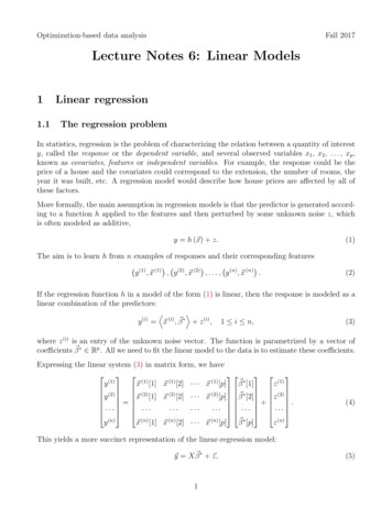
Relative coefficient error (l2 norm)0.10p 50p 100p 2000.08p1/ n0.060.040.020.0050500010000n1500020000Figure 5: Relative 2 -norm error of the least-squares coefficient estimate as n grows. The entries of X, β and z are sampled iid from a standard Gaussian distribution. The error scales as 1/ n as predictedby Theorem 2.12.Let us assume that the norm of the noise z 2 is fixed. In that case, by (48) the largest erroroccurs when z is aligned with up , the singular vector corresponding to σp , whereas the smallesterror occurs when z is aligned with u1 , the singular vector corresponding to σ1 . To analyze whathappens in a typical linear-regression problem, we can assume that X and z are sampled froma Gaussian distribution. The following theorem shows that in this case, the ratio between thenorms of the error and thepnoise (or equivalently the error when the norm of the noise is fixed toone) concentrates around p/n. In particular, for a fixed number of features it decreases as 1/ nwith the number of available data, becoming arbitrarily small as n . This is illustrated byFigure 5, which shows the results of a numerical experiment that match the theoretical analysisvery closely.Theorem 2.12 (Non-asymptotic bound on least-squares error). Let y : Xβ z,(50)where the entries of the n p matrix X and the n-dimensional vector z are iid standard Gaussians.The least-squares estimate satisfiesssrr(1 ) p(1 ) p βLS β (51)(1 ) n(1 ) n2with probability at least 1 1/p 2 exp ( p 2 /8) as long as n 64p log(12/ )/ 2 .Proof. By the same argument used to derive (49), we haveUT zσ12 1T VS U z122 UT zσp2.(52)
By Theorem 2.10 in Lecture Notes 3 with probability 1 2 exp ( p 2 /8)(1 ) p UT z22 (1 ) p,(53)where U contains the left singular vectors of X. By Theorem 3.7 in Lecture Notes 3 with probability 1 1/pppn (1 ) σp σ1 n (1 )(54)as long as n 64p log(12/ )/ 2 . The result follows from combining (52) with (53) and (54) whichhold simultaneously with probability at least 1 1/p 2 exp ( p 2 /8) by the union bound.33.1RegularizationNoise amplificationTheorem 2.12 characterizes the performance of least-squares regression when the feature matrixis well-conditioned, which means that its smallest singular value is not too small with respect tothe largest singular value.Definition 3.1 (Condition number). The condition number of a matrix A Rn p , n p, is equalto the ratio σ1 /σp of its largest and smallest singular values σ1 and σp .In numerical linear algebra, a system of equations is said to be ill conditioned if the conditionnumber is large. The reason is that perturbations aligned with the singular vector correspondingto the smallest singular value may be amplified dramatically when inverting the system. This isexactly what happens in linear regression problems when the feature matrix X is not well conditioned. The component of the noise that falls in the direction of the singular vector correspondingto the smallest singular value blows up, as proven in the following theorem.Lemma 3.2 (Noise amplification). Let X Rn p be a matrix such that m singular values aresmaller than η and let y : X β z,(55)where the entries of z are iid standard Gaussians. Then, with probability at least 1 2 exp ( m 2 /8) m 1 .(56)βLS β η2Proof. Let X U SV T be the SVD of X, u1 , . . . , up the columns of U and σ1 , . . . , σp the singular13
values. By (44)β LS β 2 V S 1 U T z2222 S 1 U T z 2 2pX uTi z σi2i(57)V is an orthogonal matrix(58)(59)m1 X T 2 2 ui z .η i(60) 2P uTi z 1 with probability at least 1 2 exp ( m 2 /8) byThe result follows because miTheorem 2.10 in Lecture Notes 3 .We illustrate noise amplification in least-squares regression through a simple example.Example 3.3 (Noise amplification). Consider a linear-regression problem with data of the form y : X β z,(61)where 0.099 0.605 0.298 0.213 0.113 X : , 0.589 0.285 0.0160.006 0.0590.032 0.212 0.471 ,β : 1.1910.066 0.077 0.010 z : . 0.033 0.010 0.028(62)The 2 norm of the noise is 0.11. The feature matrix is ill conditioned, its condition number is100, 0.234 0.427 0.674 0.202 0.241 0.744 1.00 0 0.898 0.440 .X U SV T (63) 0.654 0.350 0 0.010.4400.898 0.017 0.189 0.0670.257As a result, the component of z in the direction of the second singular vector is amplified by a14
factor of 100! By (44), the error in the coefficient estimate isβ LS β V S 1 U T z 1.000 U T z V 0 100.00 0.058 V 3.004 1.270 , 2.723(64)(65)(66)(67)so that the norm of the error satisfiesβ LS β 2 z 2 27.00.(68)4The feature matrix is ill conditioned if any subset of columns is close to being linearly dependent,since in that case there must be a vector that is almost in the null space of the matrix. This occurswhen some of the feature vectors are highly correlated, a phenomenon known as multicollinearityin the statistics ling. The following lemma shows how two feature vectors being very correlatedresults in poor conditioning.Lemma 3.4 (Proof in Section 5.2). For any matrix X Rn p , with columns normalized to haveunit 2 norm, if any two distinct columns Xi and Xj satisfyhXi , Xj i2 1 2(69)then σp , where σp is the smallest singular value of X.3.2Ridge regressionAs described in the previous section, if the feature matrix is ill conditioned, then small shifts inthe data produce large changes in the least-squares solution. In particular, some of the coefficientsmay blow up due to noise amplification. In order to avoid this, we can add a term penalizing thenorm of the coefficient vector to the least-squares cost function. The aim is to promote solutionsthat yield a good fit with small coefficients. Incorporating prior assumptions on the desiredsolution– in this case that the coefficients should not be too large– is called regularization. Leastsquares regression combined with 2 -norm regularization is called ridge regression in statistics andTikhonov regularization in the inverse-problems literature.Definition 3.5 (Ridge regression / Tikhonov regularization). For any X Rn p and y Rp theridge-regression estimate is the minimizer of the optimization problemβ ridge : arg min y X β βwhere λ 0 is a fixed regularization parameter.1522 λ β 2,2(70)
As in the case of least-squares regression, the ridge-regression estimate has a closed form solution.Theorem 3.6 (Ridge-regression estimate). For any X Rn p and y Rn we have 1 Tβ ridge : X T X λIX y .Proof. The ridge-regression estimate is the solution to a modified least-squares problem 2 yXβ ridge arg min β . β0λI(71)(72)2By Theorem 2.1 the solution equals 1 T XXβ ridge : λIλI 1 X T X λIX T y . T X y λI0(73)(74)When λ 0 then β ridge converges to the least-squares estimator. When λ , it converges tozero.The approximation X β ridge corresponding to the ridge-regression estimate is no longer the orthogonal projection of the data onto the column space of the feature matrix. It is a modified projectionwhere the component of the data in the direction of each left singular vector of the feature matrixis shrunk by a factor of σi2 / (σi2 λ) where σi is the corresponding singular value. Intuitively, thisreduces the influence of the directions corresponding to the smaller singular values which are theones responsible for more noise amplification.Corollary 3.7 (Modified projection). For any X Rn p and y Rn we have yridge : X β ridgepXσi2 h y , ui i ui ,2σ λii 1(75)(76)where u1 , . . . , up are the left singular vectors of X and σ1 . . . σp the corresponding singularvalues.Proof. Let X U SV T be the SVD of X. By the theorem, 1 TX β ridge : X X T X λIX y U SVT2T(77) T 1TV S V λV VV SU y 1 U SV T V S 2 λIV T V SU T y 1 U S S 2 λISU T y ,since V is an orthogonal matrix.16(78)(79)(80)
The following theorem shows that, under the assumption that the data indeed follow a linearmodel, the ridge-regression estimator can be decomposed into a term that depends on the signaland a term that depends on the noise.Theorem 3.8 (Ridge-regression estimate). If y : X β z, where X Rn p , z Rn andβ Rp , then the solution of Problem (70) is equal to 2σ1σ10···00···0 σ12 λ σ12 λ σ22σ2 0 0···0 T ···0 T2 λ2 λσσ22 V β V U z,β ridge V (81) ······ σp2σp00· · · σ2 λ00· · · σ2 λppwhere X U SV T is the SVD of X and σ1 , . . . , σp are the singular values.Proof. By Theorem 2.1 the solution equals 1 T X X β zβ ridge X T X λI 2 T 2 TT 1T V S V λV VV S V β V SU z 1 T V S 2 λIVV S 2 V T β V SU T z 1 2 T 1 V S 2 λIS V β V S 2 λISU T z,(82)(83)(84)(85)because V is an orthogonal matrix.If we consider the difference between the true coefficients β and the ridge-regression estimator,the term that depends on β is usually known as the bias of the estimate, whereas the term thatdepends on the noise is the variance. The reason is that if we model the noise as being randomand zero mean, then the mean or bias of the ridge-regression estimator equals the first term andthe variance is equal to the variance of the second term.Corollary 3.9 (Bias of ridge-regression estimator). If the noise vector z is random and zero mean, λ0···02 σ1 λλ 0 ···02 T σ2 λ ridge β V (86)E β V β . ··· λ00· · · σ2 λpProof. The result follows from the lemma and linearity of expectation.Increasing λ increases the bias, moving the mean of the estimator farther from the true value of thecoefficients, but in exchange dampens the noise component. In statistics jargon, we introduce biasin order to reduce the variance of the estimator. Calibrating the regularization parameter allowsus to adapt to the conditioning of the predictor matrix and the noise level in order to achieve agood tradeoff between both terms.17
2.5CoefficientsCoefficient errorLeast-squares fit2.01.51.00.50.00.5 -71010-610-510-410-310-110-2Regularization parameter100101102103Figure 6: Coefficients in the ridge-regression model (blue) for different values of the regularizationparameter λ (horizontal axis). The fit to the data improves as we reduce λ (green). The relative error ofthe coefficient estimate β β ridge / β is equal to one when λ is large (because β ridge 0), then22it decreases as λ is reduced and finally it blows up due to noise amplification (red).Example 3.10 (Noise amplification (continued)). By Theorem 3.8, the ridge-regression estimatorfor the regression problem in Example 3.3 equals 1λ00 V T β V 1 λ U T z,(87)β ridge β V 1 λλ0.010 0.012 λ0 0.012 λThe regularization λ should be set so to achieve a good balance between the two terms in theerror. Setting λ 0.01 0.001 00.99 0 V T β V U T zβ ridge β V (88)00.990 0.99 0.329 . (89)0.823The error is reduced significantly with respect to the least-squares estimate, we haveβ ridge β z 22 7.96.(90)Figure 6 shows the values of the coefficients for different values of the regularization parameter.They vary wildly due to the ill conditioning of the problem. The figure shows how least squares18
(to the left where λ 0) achieves the best fit to the data, but this does not result in a smallererror in the coefficient vector. λ 0.01 achieves a good compromise. At that point the coefficientsare smaller, while yielding a similar fit to the data as least squares.43.3Ridge regression as maximum-a-posteriori estimationFrom a probabilistic point of view, we can view the ridge-regression estimate as a maximum-aposteriori (MAP) estimate. In Bayesian statistics, the MAP estimate is the mode of the posteriordistribution of the parameter that we aim to estimate given the observed data.Definition 3.11 (Maximum-a-posteriori estimator). The maximum-a-posteriori (MAP) estimator Rm given a realization of the data vector y isof a random vector of parameters β βMAP ( y ) : arg max fβ y β y ,(91) β given the data y.where fβ y is the conditional pdf of the parameter βIn contrast to ML estimation, the parameters of interest (in our case the regression coefficients)are modeled as random variables, not as deterministic quantities. This allows us to incorporateprior assumptions about them through their marginal distribution. Ridge regression is equivalentto modeling the distribution of the coefficients as an iid Gaussian random vector.Lemma 3.12 (Proof in Section 5.3). Let y Rn be a realization of a random vector z, y : X β(92) and z are iid Gaussian random vectors with mean zero and variance σ12 and σ22 , rewhere βspectively. If X Rn m is known, then the MAP estimate of β is equal to the ridge-regressionestimateβ MAP arg min y X β β22 λ β 2,(93)2where λ : σ22 /σ12 .3.4Cross validationAn important issue when applying ridge regression, and also other forms of regularization, is howto calibrate the regularization parameter λ. With real data, we do not know the true value of thecoefficients as in Exam
Lecture Notes 6: Linear Models 1 Linear regression 1.1 The regression problem In statistics, regression is the problem of characterizing the relation between a quantity of interest y, called the response or the dependent variable, and several observed variables x 1, x 2, ., x p