WIXLIB

4Quasi-likelihood with Rsetting which uses the moment-based generalized estimating equations, see Liang and Zeger(1986). This package mostly deals with analysing clustered and longitudinal data whichtypically consist of a series of repeated measurements of usually correlated response variables.Further, the package gmm (Chaussé 2010) implements the generalized method of moments(Hansen 1982) for situations in which the moment conditions are available as closed-formexpressions. However, if the population moments are too difficult to compute, one can applythe simulated method of moments (SMM), see McFadden (1989). The moment conditions arethen evaluated as functions of the parameter by Monte Carlo simulations. Also, the packagespatstat (Baddeley, Turner, Mateu, and Bevan 2005) includes a so-called quasi-likelihoodmethod. However, the implementation is specifically made for the analysis of point processmodels.Our method is specifically designed to deal with situations where only a single measurement(i. e. ”real-world“ observation or raw data) is available and from which we can compute the(observed) summary statistics. To this end, we assume that we can define and simulate aparametric statistical model which reveals some information about the underlying data generating process. Then the parameter of interest (under this model) is inferred from a solutionto the QS equation based on these statistics. The computational complexity of our method is,therefore, mostly dominated by the effort of simulating the statistical model and evaluatingthe involved statistics. The main aim of the package is to provide an efficient implementation for generic parameter estimation problems which combines the involved statistics into atractable estimating function for simulation when no other types of parametric inference canbe applied.The vignette is organized as follows. In Section 2 we briefly present the basic theory ofQL estimation followed by an outline of the main algorithm in Section 3. We discuss someextensions of our originally proposed algorithm in Section 4. Finally, in Section 5, we providesome illustrative examples of a typical workflow of using the package.2. Basic quasi-likelihood theoryIn this section we sketch the main aspects of the general QL theory, see Heyde (1997). Let Xbe a random variable on the sample space X whose distribution Pθ depends on the unknownparameter θ Θ taking values in an open subset Θ of the q-dimensional Euclidean spaceRq . The goal is to estimate θ given the observed data x X. We assume that the familyof models Pθ is rich enough to characterise and distinguish different values of the generativeparameters. Let T : X Rp with p q be a transformation function of the data to a setof summary statistics and y T (x) is the respective (column) vector of summary statistics.We follow the QS estimating function approach to estimate θ by equating the QS Q(θ, y) Eθ [T (X)] θ tVarθ (T (X)) 1 (y Eθ [T (X])(2.1)to zero, where (·)t denotes transpose, and, respectively, Eθ and Varθ denote expectation andvariance w.r.t. Pθ .For a fixed vector of summary statistics T Rp we focus on the function G(θ, y) y Eθ [T (X)] as a vector of dimension p, for which Eθ [G] 0 for each Pθ and for which thematrices Eθ [ G/ θ] and Eθ GGt are nonsingular. The QS estimating function in (2.1) is

Markus Baaske5the standardized estimating function G̃ Eθ G θ t (Eθ GGt ) 1 G(2.2)for which the information criterionhE(G) Eθ G̃G̃ti G t Gt 1 EθEθ(Eθ [GG ]) θ θ(2.3)is maximized in the partial order of non-negative definite matrices among all linear unbiasedestimating functions of the form A(θ)(y Eθ [(T (X)], where A(θ) is any nonsingular matrix.The information criterion in (2.3) is seen as generalization of the well-known Fisher information since it coincides with the Fisher information in case a likelihood is available such thatG equals the score function in ML theory. Then, in analogy to ML estimation, the inverseof E(G) has a direct interpretation as the asymptotic variance of the estimator θ̂0 . Moreover, E(G) might serve as a measure of how much the statistics T contribute to the precisionof the estimator derived from the QS equation. Under rather minor regularity conditions,the estimator θ̂0 obtained from solving the estimating equation Q(θ̂0 , y) 0 has minimumasymptotic variance among all functions G and consistency (see, e. g. Liang and Zeger 1995)is established due to the unbiasedness assumption of the estimating equation in (2.1) whichyields, in terms of its root, a consistent estimator θ̂0 even if the covariance structure is notcorrectly specified. The information criterion in (2.3), given a vector T of summary statistics,then reads Eθ [T (X)] t 1 Eθ [T (X)]I(θ) Varθ (Q(θ, T (X))) Varθ (T (X)),(2.4) θ θwhich we call quasi-information (QI) matrix in what follows. In particular, if we had ananalytical or at least a numerically tractable form of the involved expectations and variances,we could apply a gradient based method to solve the QS equation similar to finding a rootof the score vector in ML estimation. However, since closed-form representations of expectations and variances are generally unavailable for complex statistical models or prohibitive tocompute we assume that we can only simulate realizations of the random variable X underPθ at any θ Θ.3. Simulated quasi-likelihood estimation methodLet Z : Θ Rp be a function of the model parameter θ Θ to the expected value of T , i. e.Z(θ) Eθ [T (X)], and let V (θ) Varθ (T (X)) denote the variance of the statistics under Pθ .Since we assume that we can only infer T (X) by simulated realizations of X we treat Z and Vas deterministic black box functions, which could be very expensive to evaluate in practice. Inorder to compute the QS function at θ the sample means of the statistics and the variance Vare approximated by kriging models, denoted as Ẑ and, respectively, V̂ . Since both functionscan only be evaluated with a random error due to the simulation replications of the statisticalmodel we explicitly account for the resulting approximation error in the construction of theQS function by adding the kriging prediction variances of the sample means of the statistics

6Quasi-likelihood with R(seen as a measure of predictive accuracy) to V̂ as diagonal terms (see Section 4.3). Then,the resulting approximation of the QS readsQ̂(θ, y) Ẑ 0 (θ)t V̂ (θ) 1 (y Ẑ(θ))(3.1)given the observed statistics Y y. Analogously, the approximation of the informationmatrix in (2.4) isˆ Ẑ 0 (θ)t V̂ (θ) 1 Ẑ 0 (θ),(3.2)I(θ)where Ẑ 0 Rq p denotes the Jacobian (the matrix of partial derivatives of Ẑ) which isnumerically computed by finite differences based on the kriging approximations of Z. Theincluded diagonal terms play the role of individual weights for the vector of contrasts y Ẑ(θ)in (3.1) according to the predicted error of Ẑ. Likewise, for the QI matrix in (3.2), the partialderivatives of the kriging predictor Ẑ are similarly weighted. Thus, the above QS accountsfor the noises due to the simulation replications of the statistical model. Note that, comparedto the typically high simulation effort required to obtain an estimate of the statistics, theapproximations of the QS function and QI matrix can be computed inexpensively once thekriging models have been constructed. Besides the kriging approach to approximate V thepackage additionally provides other types of variance average approximations, see Dryden,Koloydenko, and Zhou (2009), including a kernel-weighted verion based on the QI matrix.Further, the SQLE method implements two criterion functions for estimation. The first oneis directly derived from quasi-likelihood theory. The so-called quasi-deviance (QD) is definedbyˆ 1 Q̂(θ),s(θ) Q̂(θ)t I(θ)(3.3)where we suppress the dependency on the observed statistics y for convenience. In particular,the QS and QD are considered as inexpensive approximations of their respective counterpartsif T could be computed from X under the model Pθ without error at any θ D. The QD roughly speaking - measures the ”deviance“ of the QS vector from zero and thus provides aglobal view on the estimation problem with the goal of solving the QS equation. Opposed tothis, the Mahalanobis distance (MD), which readsm(θ) {y Ẑ(θ)}t Σ 1θ {y Ẑ(θ)},(3.4)where Σ is a positive definite matrix, such as an estimate of the asymptotic variance of y,has a direct interpretation as a (weighted or generalized) least squares criterion dependingon the employed type of variance matrix approximation. It can be seen as a special case ofSMM, where, in our implementation, either Σθ Σ(θ) is evaluated as a function of θ (usingMonte Carlo simulations) or considered as a ”constant“ estimate for fixed θ. In principle, bothcriterion functions can be used to guide the estimation procedure towards a (possibly local)minimum or a root of the QS function. However, in contrast to the QD, the gradient of theMD for constant Σ,m0 (θ) Ẑ 0 (θ)t Σ 1 (y Ẑ(θ)),(3.5)is readily available (ignoring irrelevant factors) and thus can be used to minimize the criterionfunction by gradient based methods. This makes the MD also desireable in terms of efficiencyand numerical stability for local searches. Obviously, in case the problem dimension equalsthe number of summary statistics, i. e. p q, both criterion functions coincide. Note thatsince the MD can be subsumed under the general term of quasi-likelihood, different versions

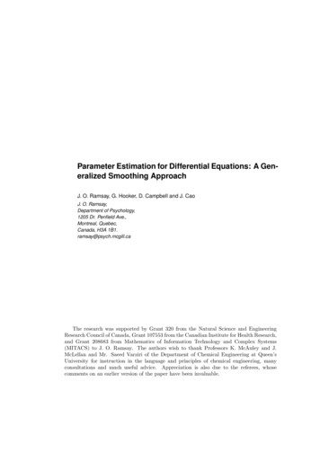
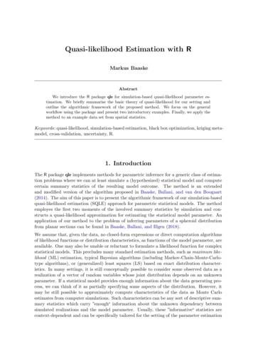
Markus Baaske7Generate design,simulate and validate models,construct QS surrogateConstruct and minimizea criterion functionCheckconvergenceand balsamplingSimulate and updateFigure 1: Algorithmic strucure of function qle(see documentation) of the MD are implemented in the package mainly for two reasons: first,the MD could be used as a preliminary step in order to identify suitable starting pointsfor parameter estimation and, secondly, to assess the goodness-of-fit of the estimated modelparameter.3.1. Algorithmic overviewAn outline of the algorithmic framework of our method is given in Figure 1. The basicalgorithm starts by generating an experimental design of size n0 of space-filling points, i. e.the parameters in our setting, and evaluates the statistics at these initial design points bysimulation. We say that an evaluated point is a point of the search space D where the statisticalmodel is simulated w.r.t. to this parameter or synonymously called ”point“. Based on thesame set of sample points and initially simulated statistics, the kriging models are separatelyconstructed for each statistic T (j) R, j 1, . . . , p so that the algorithm needs to maintainand update p kriging models simultaneously each time a new evaluation point is added. Also,the user has the option to analyse the initially generated design based on the chosen covariancestructure in terms of its adequacy for both the observed and simulated values of the statistics,the prediction accuracy and the basic assumptions of the data phenomenon (see Section 4.5).Moreover, the prediction variance for each point is used to account for the approximationerror of the QS vector depending on the current iterate θ each time the algorithm requestsa new function value of the QS or the criterion function. In particular, finding a solution to

8Quasi-likelihood with Rthe subproblems in (3.6) and (3.9) also requires to evaluate either of them.During the main iteration the algorithm updates the QS approximation and the criterionfunction based on newly evaluated design points, that is, we sequentially select new parametersof the search space for simulating the statistical model by the dual goal of improving theapproximations and, at the same time, narrowing the region of possible solutions of the QSfunction. To achieve this, the algorithm is split into a local and global phase (see Section 4.1and 4.2) as shown in Figure 1, each using its own sampling and selection criterion for newcandidates and search methods to improve the current parameter estimate. In particular, theglobal phase explores unvisited regions based on one of the criterion functions where in somesense is evidence to suspect a global or local solution to the parameter estimation problem. Onthe contrary, the local phase exploits promising local regions for small values of the criterionfunction in the vicinity of an approximate root or a minimizer. If the value of the criterionfunction drops below a user-defined tolerance at some point, we immediately switch to thelocal phase and, otherwise, continue with sampling in the global phase. Thus, the algorithmis allowed to dynamically switch the phases depending on the number of successful iterationstowards a potential parameter estimate. The proposed sampling strategies and selectioncriteria ensure that the search space becomes overall densely sampled if the algorithm isallowed to iterate infinitly often. Moreover, it keeps a ballance between global and localsearch steps which is essential for the efficiency of the method in practical applications and,at least in theory, guarantees to find a global minimum.3.2. Approximately solving the quasi-score equationThrougout this section we use the QD as the only criterion function for monitoring theestimation. We aim on estimating θ0 θ0 (T ) for given T as the parameter of the hypothesizedtrue model Pθ0 . Using Q̂ in (3.1) we deduce an estimate θ̂ D from a solution to theapproximating QS equationQ̂(θ) 0(3.6)by a Fisher quasi-scoring iteration (see, e. g. Osborne 1992). In practice, we observed thatsolving (3.6) might cause numerical instabilities for small- or medium-sized sets of (initial)sample points due to potential approximation inaccuracies of the resulting QS equation.Therefore, even if there are no roots identifiable, we aim on searching for at least an approximate (local) minimizer of one of the criterion functions and then proceed using this lastestimate. If we neither assume that equation (3.6) has a unique root nor that it exists, then,a common approach is to restrict the estimation to ”plausible“ regions of the parameter spaceas to guarantee the existence of a solution. Therefore, we define the parameter search spacebyD {θ Θ : θl θ θu } Θ,(3.7)where θl Rq and θu Rq denote the lower and upper bounds, respectively, as simple boundconstraints. In case of multiple roots, restricting to reasonably chosen smaller subregionsmight also be a pragmatic solution to distinguish between them. Another approach is givenin Section 3.4.In our implementation, the quasi-scoring algorithm is defined as a projected Newton-typeiteration with the updateˆ 1 Q̂(θ),h I(θ)(3.8)θ PD [θ αh],

Markus Baaske9where PD denotes the projection operator on D and 0 α 1 is a step size parameter for thequasi-scoring correction h Rq . In contrast to the usual setting of ML estimation the quasiscoring iteration lacks explicit values of an objective function, monitoring the progress of theiterates towards a root, because of the (in theory) left undefined quasi-likelihood function. Anatural way to measure the progress (adjusting the correction h and step length parameterα accordingly) is to use the QD as a monitor function. Therefore, the purpose of the QDis twofold: on the one hand, it is used as a surrogate objective function to monitor the rootfinding and guarantees the existence of a global minimum over D Θ. On the other hand,given the observed statistics, we can also set up a hypothesis (see Section 4.7) of the estimatedparameter to be the true one based on the approximating QS and QD as a test statistic.As a surrogate objective function, a global minimizer of the QD takes the QS closest tozero (in the limit of a sequence of surrogate minimizations) and hence is considered to bean estimate, not necessarily unique, of the unknown model parameter. However, the quasiscoring iteration might fail to converge in practice mainly for two reasons. Besides pathologicalcases, for example, if no true root exists in D, there are no theoretically backed up tests ofsome sort of sufficient decrease condition (by contrast to, for example, the Goldstein test orArmijo condition for ML estimation), which would ensure global convergence to a root of theQS by a suitable line search strategy. Therefore, we follow a hybrid search strategy in ourimplementation as follows. If the quasi-scoring iteration fails, we switch to some derivative-freeoptimization method (see, e. g. Conn, Scheinberg, and Vicente 2009) in order to approximatelysolve the QS equation because we assume that derivatives of any of the involved quantities ofthe QD are unavailable or computational prohibitive to obtain. In case of non-convergence,we search for a minimizer of the (asymptotically) equivalent optimization problemmin s(θ)(3.9)s.t. θ D.(3.10)However, the condition that h is a descent direction, particularly for the QD function, mustbe also checked to ensure a reasonable descrease after each updated correction. In order toavoid additional expensive numerical computations of function values and derivatives of theQS we implement this check as part of a line search procedure using the simple conditions(PD [θ αh]) s(θ) (3.11)of decreasing function values coupled with a backtracking algorithm, where 0 is used toensure a minimum improvement in each iteration similar to the sufficient decrease conditionin the Goldstein-Armijo rule. Further, a backtracking line search is applied on the projectionarc PD [θ αh] and hence all iterates stay within the feasable set D.3.3. Estimating the error of the quasi-score approximationAs a measure of accuracy of the QS approximation we transform the prediction variances intoan approximation error of the QS function. To this end, letB̂θ Ẑ 0 (θ)V̂ (θ) 1 Rq p(3.12)be a non-random weighting matrix given the data Y y w.r.t. to Pθ . Then, assuming B̂θand the statistical error of the QS function to be known, the QS approximation error readsĈ(θ) Var(B̂θ (y Ẑ(θ))) B̂θ Σ̂K (θ)B̂θt Rq q ,(3.13)

10Quasi-likelihood with Rwhere the variance operation is w.r.t. to the distribution of the kriging predictor Ẑ and Σ̂Kdenotes the diagonal matrix of kriging variances. Since the inverse of the QI matrix servesas an estimated statistical lower bound (like the Cramér-Rao bound in ML theory) on theestimation error of θ̂0 , we can compare the QS approximation error with the overall achievableaccuracy given by the QI matrix in (3.2). More specifically, if the largest generalized eigenvalue(see, e. g. Golub and Loan 1996), say λmax λmax (θ), of these two matrices drops below somelimit c 1 such thatĈ L c · Iˆ(3.14)holds in the Loewner partial ordering of non-negative definite matrices, we say, that the QSapproximation error is negligible compared to the predicted error of θ̂. This can be seen as anindication that no further benefit can be expected (from sampling new points) since we cannotget any better in estimating the unknown model parameter given the simulated statistics atthe current design.3.4. Termination conditionsWe define two types of termination conditions of the estimation procedure. First, the statistical stopping conditions, control the sampling process and measure the level of accuracy ofthe QS approximation and, secondly, the numerical conditions which heuristically monitorthe convergence of the sequence of approximated roots of the QS or stationary points of thecriterion function. The algorithm stops sampling new evaluation points as soon as any ofthese conditions hold and immediately terminates the estimation.The statistical conditions measure the improvement of the QS approximation achieved atiteration n. Since any criterion for stopping may strongly fluctuate

structs a quasi-likelihood approximation for estimating the statistical model parameter. An application of our method to the problem of inferring parameters of a spheroid distribution from planar sections can be found inBaaske, Ballani, and Illgen(2018). We assume that, given the data, no closed-form expressions or direct computation algorithms