Transcription
Methodological BriefsImpact Evaluation No. 8Quasi-Experimental Designand MethodsHoward White and Shagun Sabarwal
UNICEF OFFICE OF RESEARCHThe Office of Research is UNICEF’s dedicated research arm. Its prime objectives are to improveinternational understanding of issues relating to children’s rights and to help facilitate full implementation ofthe Convention on the Rights of the Child across the world. The Office of Research aims to set out acomprehensive framework for research and knowledge within the organization, in support of UNICEF’sglobal programmes and policies, and works with partners to make policies for children evidence-based.Publications produced by the Office are contributions to a global debate on children and child rights issuesand include a wide range of opinions.The views expressed are those of the authors and/or editors and are published in order to stimulate furtherdialogue on impact evaluation methods. They do not necessarily reflect the policies or views of UNICEF.OFFICE OF RESEARCH METHODOLOGICAL BRIEFSUNICEF Office of Research Methodological Briefs are intended to share contemporary research practice,methods, designs, and recommendations from renowned researchers and evaluators. The primaryaudience is UNICEF staff who conduct, commission or interpret research and evaluation findings to makedecisions about programming, policy and advocacy.This brief has undergone an internal peer review.The text has not been edited to official publication standards and UNICEF accepts no responsibility forerrors.Extracts from this publication may be freely reproduced with due acknowledgement. Requests to utilizelarger portions or the full publication should be addressed to the Communication Unit atflorence@unicef.orgTo consult and download the Methodological Briefs, please visit http://www.unicef-irc.org/KM/IE/For readers wishing to cite this document we suggest the following form:White, H., & S. Sabarwal (2014). Quasi-experimental Design and Methods, Methodological Briefs: ImpactEvaluation 8, UNICEF Office of Research, Florence.Acknowledgements: This brief benefited from the guidance of many individuals. The author and the Officeof Research wish to thank everyone who contributed and in particular the following:Contributors: Greet PeersmanReviewers: Nikola Balvin, Sarah Hague, Debra Jackson 2014 United Nations Children’s Fund (UNICEF)September 2014UNICEF Office of Research - InnocentiPiazza SS. Annunziata, 1250122 Florence, ItalyTel: ( 39) 055 20 330Fax: ( 39) 055 2033 220florence@unicef.orgwww.unicef-irc.org
Methodological Brief No.8: Quasi-Experimental Design and Methods1.QUASI-EXPERIMENTAL DESIGN AND METHODS: ABRIEF DESCRIPTIONQuasi-experimental research designs, like experimental designs, test causal hypotheses. In bothexperimental (i.e., randomized controlled trials or RCTs) and quasi-experimental designs, the programmeor policy is viewed as an ‘intervention’ in which a treatment – comprising the elements of theprogramme/policy being evaluated – is tested for how well it achieves its objectives, as measured by a prespecified set of indicators (see Brief No. 7, Randomized Controlled Trials). A quasi-experimental design bydefinition lacks random assignment, however. Assignment to conditions (treatment versus no treatment orcomparison) is by means of self-selection (by which participants choose treatment for themselves) oradministrator selection (e.g., by officials, teachers, policymakers and so on) or both of these routes.1Quasi-experimental designs identify a comparison group that is as similar as possible to the treatmentgroup in terms of baseline (pre-intervention) characteristics. The comparison group captures what wouldhave been the outcomes if the programme/policy had not been implemented (i.e., the counterfactual).Hence, the programme or policy can be said to have caused any difference in outcomes between thetreatment and comparison groups.There are different techniques for creating a valid comparison group, for example, regression discontinuitydesign (RDD) and propensity score matching (PSM), both discussed below, which reduces the risk of bias.The bias potentially of concern here is ‘selection’ bias – the possibility that those who are eligible or chooseto participate in the intervention are systematically different from those who cannot or do not participate.Observed differences between the two groups in the indicators of interest may therefore be due – in full orin part – to an imperfect match rather than caused by the intervention.There are also regression-based, non-experimental methods such as instrumental variable estimation andsample selection models (also known as Heckman models). These regression approaches take account ofselection bias, whereas simple regression models such as ordinary least squares (OLS), generally do not.There may also be natural experiments based on the implementation of a programme or policy that can bedeemed equivalent to random assignment, or to interrupted time series analysis, which analyses changesin outcome trends before and after an intervention. These approaches are rarely used and are notdiscussed in this brief.Methods of data analysis used in quasi-experimental designs may be ex-post single difference or doubledifference (also known as difference-in-differences or DID).Main pointsQuasi-experimental research designs, like experimental designs, test causal hypotheses.A quasi-experimental design by definition lacks random assignment.Quasi-experimental designs identify a comparison group that is as similar as possible to thetreatment group in terms of baseline (pre-intervention) characteristics.There are different techniques for creating a valid comparison group such as regressiondiscontinuity design (RDD) and propensity score matching (PSM).1Shadish, William R., et al., Experimental and Quasi-Experimental Designs for Generalized Causal Inference, Houghton MifflinCompany, Boston, 2002, p. 14.Page 1
Methodological Brief No.8: Quasi-Experimental Design and Methods2.WHEN IS IT APPROPRIATE TO USE QUASIEXPERIMENTAL METHODS?Quasi-experimental methods that involve the creation of a comparison group are most often used when it isnot possible to randomize individuals or groups to treatment and control groups. This is always the case forex-post impact evaluation designs. It may also be necessary to use quasi-experimental designs for ex-anteimpact evaluations, for example, where ethical, political or logistical constraints, like the need for a phasedgeographical roll-out, rule out randomization.Quasi-experimental methods can be used retrospectively, i.e., after the intervention has taken place (attime t 1, in table 1). In some cases, especially for interventions that are spread over a longer duration,preliminary impact estimates may be made at mid-term (time t, in table 1). It is always highly recommendedthat evaluation planning begins in advance of an intervention, however. This is especially important asbaseline data should be collected before the intended recipients are exposed to the programme/policyactivities (time t-1, in table 1).Timing of intervention and data collection for impact evaluations with alarge sample -1tt 1Baseline(Mid-term survey)Endlinet a specific time period3.QUASI-EXPERIMENTAL METHODS FOR CONSTRUCTINGCOMPARISON GROUPSPropensity score matching (PSM)What is matching?Matching methods rely on observed characteristics to construct a comparison group using statisticaltechniques. Different types of matching techniques exist, including judgemental matching, matchedcomparisons and sequential allocation, some of which are covered in Brief No. 6, Overview: Strategies forCausal Attribution. This section focuses on propensity score matching (PSM) techniques.Perfect matching would require each individual in the treatment group to be matched with an individual inthe comparison group who is identical on all relevant observable characteristics such as age, education,religion, occupation, wealth, attitude to risk and so on. Clearly, this would be impossible. Finding a goodmatch for each programme participant usually involves estimating as closely as possible the variables ordeterminants that explain the individual’s decision to enrol in the programme. If the list of these observablecharacteristics is very large, then it becomes challenging to match directly. In such cases, it is moresuitable to use PSM instead.Page 2
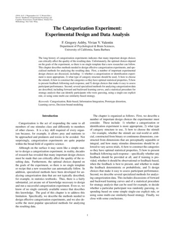
Methodological Brief No.8: Quasi-Experimental Design and MethodsWhat is PSM?In PSM, an individual is not matched on every single observable characteristic, but on their propensityscore – that is, the likelihood that the individual will participate in the intervention (predicted likelihood ofparticipation) given their observable characteristics. PSM thus matches treatment individuals/householdswith similar comparison individuals/households, and subsequently calculates the average difference in theindicators of interest. In other words, PSM ensures that the average characteristics of the treatment andcomparison groups are similar, and this is deemed sufficient to obtain an unbiased impact estimate.How to apply PSMPSM involves the following five steps:1. Ensure representativeness – Ensure that there is a representative sample survey of eligibleparticipants and non-participants in the intervention. Baseline data are preferred for calculatingpropensity scores. This technique can, however, also be used with endline data: the matchingvariables must be variables that are unaffected by the intervention.2. Estimate propensity scores – The propensity scores are constructed using the ‘participationequation’, which is either a logit or probit regression with programme participation as the dependentvariable (in the programme 1, not in the programme 0). The characteristics deemed to affectparticipation should be well considered and as exhaustive as possible, but should excludecharacteristics that may have been affected by the intervention. For this reason, it is best to usebaseline data, where available, to estimate the propensity scores.3. Select a matching algorithm – Each member of the treatment group is then matched to one ormore members of the comparison group. There are different ways of doing this such as matchingeach participant to their ‘nearest neighbour’ non-participant. The mean of the closest five neighboursis most commonly used.A single individual in the comparison group may be matched to several different individuals in thetreatment group.In order for the matching to be valid, it is essential to compare ‘observed values’ for participants andnon-participants with the same range of characteristics. Observations in the comparison group with apropensity score lower than the lowest observed value in the treatment group are discarded.Similarly, observations in the treatment group with a propensity score higher than the highestobserved value in the comparison group are also discarded. What remains is known as ‘the region ofcommon support’ – an example is detailed in figure 1.Page 3
Methodological Brief No.8: Quasi-Experimental Design and MethodsFigure 1. Example of a distribution of propensity scores – region of common support is 0.31to 0.80Source: Data created by authors for illustrative purposes only.Figure 1 shows a typical distribution of propensity scores. The distribution for the treatment group isto the right of that of the comparison group – that is, treatment group individuals tend to have higherpropensity scores than those in the comparison group. No member of the treatment group has apropensity score of less than 0.3, and no member of the comparison group has a propensity score ofmore than 0.8. So, in establishing the region of common support, the 39 per cent of comparisongroup observations with a propensity score of 0 to 0.3 are ignored, along with the 19 per cent oftreatment group observations with a propensity score of 0.8 to 1. (In practice, a more precise cut-offwould be used than that shown by the categorical classification of the data.)Table 2 shows the matching for selected variables from a PSM analysis for a study of the impact ofaccess to clean water in Nepal.2 The ‘before matching’ column compares the average characteristicsof households with access to clean water in the treatment group compared to all those householdswithout access to clean water in the comparison group. These two groups of households are verydifferent: those with access to clean water are more likely to be urban, better educated and better offthan those without access to clean water. Any difference in child diarrhoea between the two groupscannot be readily attributed to access to clean water, however, since there are many otherdifferences that may explain why the incidence of child diarrhoea varies between the groups.2Bose, Ron, ‘The impact of Water Supply and Sanitation interventions on child health: evidence from DHS surveys’, conferencepaper, Bi-annual Conference on Impact Evaluation, Colombo, Sri Lanka, 22 to 23 April 2009.Page 4
Methodological Brief No.8: Quasi-Experimental Design and MethodsObservable characteristics before and after matching (percentage of group displaying thecharacteristic)Before matchingVariableAfter rison(%)Rural resident29783338Richest wealth quintile4623936Household head highereducation2141717Source: Bose, Ron, ‘The impact of Water Supply and Sanitation interventions on child health: evidence from DHSsurveys’, conference paper, Bi-annual Conference on Impact Evaluation, Colombo, Sri Lanka, 22 to 23 April 2009.Following matching, the differences between the two groups are substantially reduced. Establishingthe region of common support discards those households without access to clean water who are verydissimilar to those with access to clean water, so households in the matched comparison group aremore urban, better educated and better off than households without access to clean water as awhole. Similarly, the least similar members of the treatment group have also been discarded from theevaluation.4. Check for balance – The characteristics of the treatment and comparison groups are compared totest for balance. Ideally, there will be no significant differences in average observable characteristicsbetween the two groups. Now that the treatment and comparison groups are similar on observablecharacteristics, variance in the incidence of child diarrhoea between the treatment and comparisongroups can be attributed to differences such as access to clean water.5. Estimate programme effects and interpret results – Finally, the impact estimate, either single ordouble difference, is calculated by firstly calculating the difference between the indicator for thetreatment individual and the average value for the matched comparison individuals, and secondlyaveraging out all of these differences.Table 3 shows an example (with nearest neighbour matching) using data on learning outcomes forgrade (or year) six children on a standardized test. Column 1 shows the test score for individualsfrom the treatment group, and columns 4 to 8 show the test score for the nearest five neighbours ofeach from the comparison group. The average score for the five neighbours is shown in column 2,and the difference between the treatment individual’s test score and this average is shown in column3. The single difference impact estimate is the average of the values in column 4.Page 5
Methodological Brief No.8: Quasi-Experimental Design and MethodsCalculation of the propensity score impact estimate: Example using test score 37.2569.059.79.355.657.657.162.465.8 .239.138.740.137.5Average52.945.57.4Observed(i)In practice, these calculations do not need to be done manually as statistical packages (e.g., Stata, SAS orR) are available to conduct the analysis.What is needed to conduct PSM?PSM requires data from both the treatment group and a potential comparison group. Both samples must belarger than the sample size suggested by power calculations (i.e., calculations that indicate the sample sizerequired to detect the impact of an intervention) since observations outside the region of common supportare discarded. Generally, oversampling must be greater for the potential comparison group than for thetreatment group.PSM can be conducted using data from surveys, administrative records, etc. The data for the treatmentand comparison groups may come from different data sets provided that: (1) they contain data on the samevariables (i.e., defined in the same way); and (2) the data were collected during the same time frame. Thelatter requirement is particularly important for seasonal variables – that is, variables that are sensitive to thedifferent seasons such as weight for age.Advantages and disadvantages of PSMThe two main advantages of PSM are that it is always feasible if data are available, and it can be doneafter an intervention has finished, including in the absence of baseline data (although this is not ideal). Ifbaseline data are unavailable, ‘recall’ can be used to reconstruct pre-intervention characteristics. This canbe imprecise, however, and common sense should prevail when deciding which variables can be recalledaccurately.The main drawback is that PSM relies on matching individuals on the basis of observable characteristicslinked to predicted likelihood of participation. So, if there are any ‘unobserved’ characteristics that affectparticipation and which change over time, the estimates will be biased and thus affect the observed results.Page 6
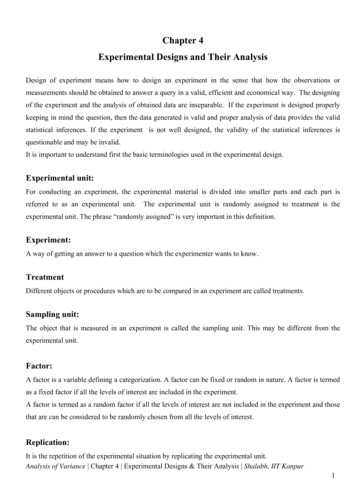
Methodological Brief No.8: Quasi-Experimental Design and MethodsAn additional practical limitation of using PSM is the need for the assistance of a statistician or someonewith skills in using different statistical packages.Regression discontinuity design (RDD)What is RDD?This approach can be used when there is some kind of criterion that must be met before people canparticipate in the intervention being evaluated. This is known as a threshold. A threshold rule determineseligibility for participation in the programme/policy and is usually based on a continuous variable assessedfor all potentially eligible individuals. For example, students below a certain test score are enrolled in aremedial programme, or women above or below a certain age are eligible for participation in a healthprogramme (e.g., women over 50 years old are eligible for free breast cancer screening).Clearly, those above and below the threshold are different, and the threshold criterion (or criteria) may wellbe correlated with the outcome, resulting in selection bias. Remedial education is provided to improvelearning outcomes, and therefore those with poorer learning outcomes are picked to be in the programme.Older women are more likely to get breast cancer, and it is older women who are selected for screening.So, simply comparing those in the programme with those not in the programme will bias the results.Those just either side of the threshold are not very different, however. If the threshold for being enrolled ina remedial study programme is a test score of 60, students enrolled in the programme who get a score of58 to 59.9 are not very different from those who get a score of 60 to 60.9 and are not enrolled. Regressiondiscontinuity is based on a comparison of the difference in average outcomes for these two groups.How to apply RDDThe first step is to determine the margin around the threshold and this is done using an iterative approach.At first, a small margin can be set up, and the resulting treatment and comparison groups can be tested fortheir balance or similarity. If the match is good, the margin can be widened a little and the balance checkedagain. This process must be repeated until the samples start to become dissimilar. Although balancing isbased on observable characteristics, there is no reason to expect imbalance among non-observablecharacteristics (this is different in the case of PSM, as explained above).Once the sample is established, a regression line is fitted. This is a line drawn through the data pointsthat represents the ‘best fit’ between the variables being studied or that summarizes the‘relationship’ between the selected variables – that is, when the line slopes down (from top left tobottom right) it indicates a negative or inverse relationship; when it slopes up (from bottom left to top right)a positive or direct relationship is indicated. In this case, the regression line is fitted on the selectedoutcome of interest (e.g., test scores). The sample for the regression is restricted to observations just eitherside of the threshold. Often a major challenge for RDD is the need for sufficient observations on either sideof the threshold to be able to fit the regression line.An example of a remedial education programme is shown in figure 2. The selection criterion for eligibility toparticipate in the programme is a pre-intervention test score, with a threshold of 60. The outcome variableis a post-intervention test score. The scatter plot shows that these two variables are, unsurprisingly,related. There is a positive relationship between pre- and post-intervention test scores. Children with a preintervention test score of below 60 received the remedial classes. The sample used for the analysis istaken from just either side of the threshold – those included have pre-intervention test scores in the rangeof 50 to 70, i.e., 10 units either side of the threshold. The fitted regression line has a ‘jump’; this is thediscontinuity. The size of this jump (which is 10) is the impact of the programme – that is, the remedialeducation programme increases test scores by 10 points on average.Page 7
Methodological Brief No.8: Quasi-Experimental Design and MethodsRegression discontinuity designPost-intervention test scoreFigure 2.What is needed for RDD?Data are required on the selection variable and the outcome indicator for all those considered for anintervention, whether accepted or not. Many programmes do not keep information on individuals refusedentry to the programme, however, which can make RDD more difficult.Advantages and disadvantages of RDDRDD deals with non-observable characteristics more convincingly than other quasi-experimental matchingmethods. It can also utilize administrative data to a large extent, thus reducing the need for data collection– although the outcome data for those not accepted into the programme often need to be collected.The limits of the technique are that the selection criteria and/or threshold are not always clear and thesample may be insufficiently large for the analysis (as noted above). In addition, RDD yields a ‘local areatreatment effect’. That is, the impact estimate is valid for those close to the threshold, but the impact onthose further from the threshold may be different (it could be more or less). In practice, however, where ithas been possible to compare this ‘local’ effect with the ‘average’ effect, the differences have not beengreat. This indicates that RDD is an acceptable method for estimating the effects of a programme or policy.Epidemiological approachesEpidemiologists apply a range of statistical data collected from treated and untreated populations, includingordinary least squares and logistic regressions in the case of dichotomous outcomes (having thecondition 1, not having the condition 0). When using these methods, it is preferable to: (1) use datafrom well matched treatment and comparison groups, and (2) restrict the regression analysis toobservations from the region of common support. (These steps are not usually taken at present, however.)Page 8
Methodological Brief No.8: Quasi-Experimental Design and MethodsSome epidemiological studies present the difference in means between treated and untreatedobservations, but this approach does not take account of possible selection bias.Survival analysis can be an appropriate approach when data are censored, meaning that the period ofexposure is incomplete because of the timing of data collection or the death of the study participant. TheCox proportional hazards model is commonly used in such circumstances.4.QUASI-EXPERIMENTAL METHODS FOR DATA ANALYSISSingle difference impact estimatesSingle difference impact estimates compare the outcomes in the treatment group with the outcomes in thecomparison group at a single point in time following the intervention (t 1, in table 1).Difference-in-differencesWhat is erences (DID), also known as the ‘double difference’ method, compares the changes inoutcome over time between treatment and comparison groups to estimate impact.DID gives a stronger impact estimate than single difference, which only compares the difference inoutcomes between treatment and comparison groups following the intervention (at t 1). Applying the DIDmethod removes the difference in the outcome between treatment and comparison groups at the baseline.Nonetheless, this method is best used in conjunction with other matching methods such as PSM or RDD. IfDID is used without matching, the researchers should test the ‘parallel trends assumption’, i.e., that thetrend in outcomes in treatment and comparison areas was similar before the intervention.Below is a hypothetical example of the DID method. Table 4 shows data for nutritional status, as measuredby weight-for-age z-scores (WAZ), for treatment and comparison groups before and after a programme ofnutritional supplementation.Child nutritional status (WAZ) for treatment and comparison groups at baseline andendlineBaselineEndlineChangeTreatment (Y1)-0.66-0.48 0.18Comparison (Y0)-0.62-0.58 0.04 0.10 0.14DifferenceThe magnitude of impact estimated by the single and double difference methods is very different. Thesingle difference (SD) estimate is difference in WAZ between treatment and comparison groups followingthe intervention, that is, SD -0.48 – (-0.58) 0.10. The DID estimate is the difference in WAZ of thetreatment group at the baseline and following the intervention minus the difference in WAZ of thecomparison group at the baseline and following the intervention, that is, DID [-0.48 – (-0.66)] – [-0.58 – (0.62)] 0.18 – 0.04 0.14.Page 9
Methodological Brief No.8: Quasi-Experimental Design and MethodsThe double difference estimate is greater than the single difference estimate since the comparison grouphad better WAZ than the treatment group at the baseline. DID allows the initial difference in WAZ betweentreatment and comparison groups to be removed; single difference does not do this, and so in this exampleresulted in an underestimate of programme impact.How to apply the DID methodThe first step involves identifying the indicators of interest (outcomes and impacts) to be measured relevantto the intervention being evaluated. Following this, the differences in indicator values from before and afterthe intervention for the treatment group are compared with the differences in the same values for thecomparison group. For example, in order to identify the effects of a free food scheme on the nutritionalstatus of children, the mean difference for both the treatment group and the comparison group would becalculated and then the difference between the two examined, i.e., by looking at the difference betweenchanges in the nutrition status of children who participated in the intervention compared to those who didnot. Ideally, the intervention and comparison groups will have been matched on key characteristics usingPSM, as described above, to ensure that they are otherwise as similar as possible.Advantages and disadvantages of the DID methodThe major limitation of the DID method is that it is based on the assumption that the indicators of interestfollow the same trajectory over time in treatment and comparison groups. This assumption is known as the‘parallel trends assumption’. Where this assumption is correct, a programme impact estimate made usingthis method would be unbiased. If there are differences between the groups that change over time,however, then this method will not help to eliminate these differences.In the example above, if the comparison states experienced some changes that affect the nutritional statusof children – following the start of the free food scheme in other states – then the use of DID alone wouldnot provide an accurate assessment of the impact. (Such changes might occur, for example, because ofdevelopment programmes that raise the income levels of residents, meaning they can afford to give theirchildren a more nutritious diet.)In summary, DID is a good approach to calculating a quantitative impact estimate, but this method alone isnot usually enough to address selection bias. Taking care of selection bias requires matching to ensurethat treatment and comparison groups are as alike as possible.Regression-based methods of estimating single and double difference impact estimateSingle and double difference impact estimates may also be estimated using ordinary least squaresregression. This approach is applied to the same matched data, including a programme or policy dummyvariable on the right-hand side of the regression equation. Variables that capture other confounding factorscan also be included on the right-hand side to eliminate the remaining effect of any discrepancies in thesevariables between treatment and comparison areas on the outcomes after matching.5.ETHICAL ISSUES AND PRACTICAL LIMITATIONSEthical issuesQuasi-experimental methods offer practical options for conducting impact evaluations in real world settings.By using pre-existing or
Methodological Brief No.8: Quasi-Experimental Design and Methods Page 2 2. WHEN IS IT APPROPRIATE TO USE QUASI-EXPERIMENTAL METHODS? Quasi-experimental methods that involve the creation of a comparison group are most often used when it is