Transcription
Advanced Transform MethodsProfessor Sir Michael Brady FRS FREngDepartment of Engineering ScienceOxford UniversityHilary Term 2006
Outline Recap on Fourier domainLimitations of the Fourier transformGabor’s great ideaAnalytic signal, local phase & featuresBases for spaces of functionsWaveletsThe Riesz transform, monogenic signal &features again
Recap on Fourier domain Frequency for signal/image processing– “Frequency freaks” vs “feature creatures” Fourier’s idea– Was using sine/cosine lucky or insightful? Efficiency: the FFTThe importance of phaseHomomorphic filteringImage enhancement & restoration
Frequency for signal/imageanalysis “noise” is often high frequency– Unfortunately, so are transients such as edges, corners, – The human visual system ignores constant signals but detectssignal changes– Filtering out high frequencies can damage edges Textures often have repeated patterns that correspondto peaks in Fourier spectrum– Unfortunately, this is too simple for texture analysis in practice Frequency codes for position in MRI Sadly, Fourier theory is often ignored in image analysis –at cost of poorer results than necessary– Example of rotational invariance of feature detection
Frequency freaksSinusoidalgratingCampbell and Robson’scontrast sensitivity functionCSFOutput from the monogenic signalExample of a CSF: thresholdcontrast vs spatial frequency(cycles/degree or lp/mm)
a. Corners detected by aconventional algorithmas a shape rotates;c. Edges detected by theCanny edge detector asthe shape rotatesb. Corners detected afterFourier analysis of thefilter response isanalysed as a function oforientation, leading to afilter whose response isanisotropicd. Edges after similaranalysisSource: DPhil thesis byJason Merron, 1997
Fourier’s idea (1807)Fourier presented a memoir to the Institut de France in which he claimed thatall continuous functions of a real variable f(t) can be represented as series ofharmonically related sines and cosines. The complete mathematical story wasnot worked out until 1960!Definition: Let f(t) be a continuous function of a real variable t, then the FourierTransform of f is defined to be: ℑ( f ) : u f (t )e jut dt Note that ℑ is an operator that transforms a function f of one variable intoanother:ℑ :L (ℜ) L (ℜ)11where L1 (ℜ) is the (Hilbert) space of integrable functions, that is : f(t) dt
Inverse FT usually existsNotation : denote ℑ( f ) by fˆAn important result is that for most functions f and for most t the inversetransform exists too:If f L1 (ℜ), then for almost all t ℜ,1f (t ) 2π fˆ (u )e jut du
Power and phaseNote that fˆ (u ) is a complex valued function fˆ (u ) fˆr (u ) jfˆi (u )Express in exponential form : fˆ (u ) fˆ (u ) e jφ (u )wherefˆ (u ) ˆf 2 (u ) fˆ 2 (u )rifˆi (u )tan φ (u ) fˆ (u )rThe first of these is the square root of the power spectrum of f, thesecond is the phase angle of f.Most of signal processing is concerned with the power spectrum;but (as we shall see) phase dominates in image analysis
Decomposing an image into itsspatial frequency components
Rectangle function and sincRectangle function plays a key role in image/signal processing.In the frequency domain it defines a perfect bandpass filter, inthe space domain a perfect windowing operator.1 1, x 2f ( x) 1 0, x 2 sin(πXu ) Xsinc(πXu )F (u ) X(πXu )Sinc interpolation plays an important role in MRI image analysis, andgeometric alignment of data sets.
Fourier transform propertiespropertyf (t )fˆ (t )fˆ (u )2πf ( u )1 ˆConvolution(h f )(t )h(u ) fˆ (u )2π jt 0u ˆTranslationf (t t0 ) ef (u )Modulatione ju0tfˆ (u u0 )tScalings fˆ ( su )f( )sTime derivativef p (t )( ju ) p fˆ (u )Frequency derivative ( jt ) pfˆ p (u )Inverse
Examples, and a questionA reminder from the FT course:cos λt1(δ (ω λ ) δ (ω λ ) )2Π (t )sincδ (t )1ω2OK, so “all continuous functions of a real variable f(t) can berepresented as series of harmonically related sines and cosines”But was Fourier's observation just lucky? Or, is there a deeperreason why cosines and sines - complex exponentials - should playa key role?
Linear, time invariant filteringAn operator L is linear if L(αf βg ) αL( f ) βL( g )for any constants α , βLinearity is a simplifying assumption that is made throughout much ofengineering science, even if it rarely holds exactly.An operator L is called time invariant if the input to f is delayed by a time τ ,then the output is also delayed by τ . That is, if fτ (t) f (t τ ), thenL( f )(t τ ) L( fτ )(t )
linear, time-invariant operators:impulses and convolutionDenote by δ (t ) the Dirac function 1 t 1δ (t ) 0 t 1and denote δ u (t ) δ (t u )Linear, time-invariant systems are characterised by their response toDirac functions. Assume for the moment that the following integrations are defined:f (t ) f (u )δ u (t )dt Linearity implies Lf (t ) f (u )Lδ u(t )dt
Impulse responseThe impulse response h of the linear, time-invariant operator L ish(t ) Lδ (t )time invariance proves that Lδ u (t ) h(t u ), so that Lf (t ) f (u )h(t u )du h(u ) f (t u )du (h f )(t )The impulse response function of a linear time-invariant operator is aconvolution
complex exponentials are eigenfunctions ofconvolution operators Le jwt h(u )e jw( t u ) du e jwt h(u )e jwu du hˆ( w)e jwt The eigenvalue hˆ( w) h(u )e jwu du is the FT of h at the frequency ω so linearity Î impulse response Î convolution Î sines & cosinesSo Fourier's insight was deep, though it may also have been lucky!
Convolution theorem and FFTWe have seen that linear, time-invariant operators correspond preciselywith those defined by convolution. That is, L is a linear, time-invariantoperator if, and only if, there is a function h(t), called the impulseresponse function of L so that Lf h*f.The convolution theorem is the core of the application of Fourier theoryto signal and image processing, since the naïve shift-and-multiplyimplementation of convolution is intrinsically expensive, havingcomplexity O(N2) where N is the desired number of values of u.Convolution Theorem : If f L1 (ℜ) and h L1 (ℜ), then h f L1 (ℜ) and (h * f ) hˆfˆConvolution in the time/space domain multiplication in Fourier domain
Practical importance of theconvolution theoremSmoothing an image with a Gaussian kernel. Could do it inthe space domain, using separability of the Gaussian, OR1. Compute the FT of the image and of theGaussian kernel2. Multiply their FTsf ( x, y ) g ( x, y ) F (u , v)G (u, v)3. Compute inverse FT of productThis only makes sense because there is a FAST FT algorithm
The FFTˆf (t ) 1NN 1 f (t )et 0 jutN1 NN 1 t 0f (t )WNutAssume N 2n for some n, so that N 2M for some M.Substituting:1 1fˆ (u ) 2 MSo that:M 1 t 0[1f (2t )WMut MM 1 t 0 f (2t 1)WMutW2uM ˆf (u ) 1 fˆ (u ) fˆ (u )W uevenodd2M2]
FFT algorithmGiven a signal {f(0), f(1), ., f(63)}, it is broken down in to: {f(0), f(2), , f(62)} and {f(1), f(3), , f(63)That is, the FT of a signal of length 64 can be computed from two FTs oflength 32. These in turn are broken down in to their odd and even bits{f(0), f(4), }; {f(2), f(6), }; {f(1), f(5), }; {f(3), f(7),.}So it can be computed from 4 of length 16. In general, For a signal oflength N, the algorithm takes time N log N instead of N2 by the naïvemethod.There is nothing magical about this process, it follows from simpleproperties of sines and cosines. Exactly, the same idea works forwavelets
2D FTIf f ( x, y ) is continuous and integrable, and if fˆ (u , v) is integrable,then we can definefˆ (u , v) f ( x, y )e j ( ux vy ) dxdy f ( x, y ) fˆ (u , v)e j ( ux vy ) dudv We can define the power and phase as for 1D FT
FT pair in 2DvF (u , v) XYsnc(πXu ) snc(πYv)
FT of a circular disk 1, r af ( x, y ) 0, r aF (u , v) F ( ρ ) aJ1 (πaρ ) / ρ2D version of a sinc functionImportant in ultrasound imageanalysis
2D FT of an X shape
Discrete FTThe function f (t ) is sampled into f (t0 nT ). A discrete sample f (nT ) correspondsto a weighted Dirac sum :f d (t ) f (nT )δ (t nT )n Using the translation theorem, and the fact that the FT of a delta is 1, we find :fˆd (u ) f (nT )e jnuTn Theorem The FT of the discrete signal obtained by sampling f uniformly at intervals T is : 12 nπ)fˆd (u ) fˆ (u T n TThis shows that sampling f at intervals T is equivalent to making itsFourier transform periodic by summing all its translations.
Discrete image filteringThe properties of 2D space-invariant operators are essentially the sameas in 1D. A linear operator L is space-invariant if, for anyf p ,q (n, m) f (n p, m q ), thenLf p ,q (n, m) Lf (n p, m q )An image can be decomposed as a sum of discrete Diracs and thenlinearity and space-invariance proves that any L has an associatedimpulse response function h(n,m) so that application of L isequivalent to a 2D convolution with h
SeparabilityThe impulse response function h(n,m) is separable if it is a product oftwo one-dimensional functions:h(n, m) h1 (n)h2 (m)In the case of a separable impulse response function, the twodimensional convolution can be rewritten as a 1D convolution alongthe columns followed by a 1D convolution along the rows (or viceversa). ( f h )(n, m) h1 (n p) h2 (m q) f ( p, q) p q Reduces compute complexity to O(2N); the discrete FT can becomputed by column then by row.Example: Gaussian convolution and pipeline architectures
FT of a Gaussianf (r ) 12πσ 2e r 2 / 2σ 2F (u, v) F ( ρ ) e, r 2 x2 y2 2π 2 ρ 2σ 2, ρ 2 u 2 v2 FT of a Gaussian is a Gaussian Note the inverse scale relation
Power spectrum of FT of an imageoriginalf(x,y) F(u,v) Low passHigh pass
Image with periodic structuref(x,y) F(u,v) FT has peaks at spatial frequencies of repeated textures
Forensic application F(u,v) Removepeaks,equalsperiodicbackground
Energy and PhaseSeems like phasecarries lessinformation aboutthe image
The importance of phaseOppenheim’s demonstrationI1I2FFTIˆ1 (u , v) P1 (u , v)e jΦ1 ( u ,v )FFTIˆ2 (u , v) P2 (u , v)e jΦ 2 ( u ,v )Iˆ3 (u , v) P1 (u , v)e jΦ 2 (u ,v )FFT-1I3Do you see: I1,I2, neither, orboth?
KebleAnotherdinosaurKeble phasesthe dinosaur
KebleAnotherdinosaurthe dinosaurphases Keble
intensityStep edge detection bydifferentiationSignal position, xProfile of a step intensity changesuperimposed on a ramp
intensityd intensity/ dxBasic feature detection conventional approachSignal position, xProfile of a step intensity changesuperimposed on a rampConstant gradient max at thestep. Note amplified noise
Differentiation as convolutionApproximate differentiation as central difference:df ( x)f (i 1) f (i 1) dx x i2Differentiation by the central difference isequivalent to convolution with the odd symmetrickernel1 1 2 ,0, 2 Problem is that differentiation amplifies noise, suggestingpre-filtering the image with a noise reducing, smoothingfilter
Convolution with the derivative of aGaussianStep detection by finding“significant” maxima of theconvolution of the signal with aderivative of a GaussiandGσ ( x) f ( x)dxStep superimposed on a ramp signal take second derivative
Gaussian derivatives in 2D x ( x 2 y 2 ) / 2σ 2 G ( x, y ) f ( x, y ) e f ( x, y )4 x 2πσ Gaussian isseparable: equivalent x xto convolution in the e32πσ x-direction and then inthe y-direction2/ 2σ 2 1 y 2 / 2σ 2 e f ( x, y ) 2π σ Directional derivative of Gaussian shown as a surface
ExampleX-derivativeY-derivative
Gradient magnitude
intensityd2 intensity/ dx2Basic feature detection –zero crossingsSignal position, xProfile of a step intensity changesuperimposed on a rampZero crossing at step. Butdoubly amplified noise
Gaussian scale spaceThis shows a Gaussian blurredsignal Gσ*S(t) as σ increases(from bottom to top)The positions of the zerocrossings of the secondderivative of the blurredsignal are marked. Thisproduces a “fingerprint”
Homomorphic filteringIllumination model: i(x,y) illum(x,y)reflec(x,y) where i(x,y)is the image, illum(x,y) is the spatially slowly-varying illumination,and reflec(x,y) is the reflectance of visible surfaces, assumedpiecewise constant.Taking logs to convert to a sum (indicated by Capitalised names),then apply the FT: Iˆ(u , v) Illum(u, v) Reflec(u, v)Apply a suitable filter H (u, v) and then take inverse FT : 1 1 Enh( x, y ) ℑ ( H (u, v) Illum(u , v)) ℑ ( H (u , v) Reflec(u , v))Then the enhanced image is obtained by taking exponents of thisequation.
Homomorphic filtering: exampleLeft: Original image. Right: processed using homomorphic filteringto achieve contrast enhancement and dynamic range compression.
Homomorphic filtering in practice The choice of the filter H(u,v) is critical– it must affect low and high frequencies in differentways– illumination varies spatially slowly'' suggests lowpass– H(u,v) is typically 1-Butterworth'' Note that noise was ignored Worse, reflectance also has a low frequencycomponent, so separation is often hard– bias field'' in MRI image enhancement
Signal/image restoration using theFourier domainThe objective is to restore a degraded image to its original form. Anobserved image can often be modelled as:g ( x, y ) h ( x, y ) f ( x, y ) n ( x, y )where f is the signal/image to be restored, h is the point spread functionof the imaging process, n is additive noise, and g is the signal/imagewith which we are confronted. The aim is to restore f given g and someknowledge of n and h. Evidently: gˆ (u , v) hˆ(u , v) fˆ (u , v) nˆ (u , v) ˆIgnoring n for the moment, an estimate f of fˆ is given by : gˆ n gˆf or, re - introducing noise : f hˆhˆ hˆEvidently, problems if hˆ 0 or ĝ is small, so noise dominates
Wiener filter f (u , v) gˆ (u , v) wˆ (u , v), wherehˆ* (u , v)wherewˆ (u , v) hˆ(u , v) 2 k (u , v)k (u , v) Sη (u , v) / S f (u , v)2Sη (u , v) nˆ (u , v) is the power spectral density of the noise2 S f (u , v) f (u , v) is the power spectral density of the signal If k (u , v) 0, then f (u , v) 1 / hˆ(u, v) (ie inverse filter)if k (u , v) hˆ(u , v) for large u , v then high frequencies are attenuatedOften S f , Sη are known approximately, or k is set equal to a suitable constant
Wiener filter exampleHere, K is set to the constant value indicated
Inadequacies of the FT & attemptsto overcome them The discrete world, signal changes,localisation Localisation vs SNR Gaussian “scale space” Isotropic and anisotropic diffusion forimage analysis Estimating orientation in images :steerable filters
The transient worldA sine function with a smalldiscontinuity.The Fourier Transform consists oftwo delta functions, indicating thesingle dominant signal.Note the infinite tiny wiggles –across the entire spectrum.It detects that there is adiscontinuity; but cannot say where
The basic problem with the FT forsignal/image processingUsing the FT of the Rect function, we see that the FT of any functionthat is bounded in time, f (t ) 0, for t tlower or t tupperhas frequencies over an infinite range. Conversely, the inverse FT of aperfect band-pass filter has temporal components over an infinite range.We may detect that a transient has occurred; but we cannot detect when!If we are to treat transients in signal/image processing, we must find away to overcome this problem. (The great idea in MRI is to add agradient field to provide localisation; but that is infeasible for most signaland image processing.)
Space/time & frequency Shannon (1943) Fourier (1807)– the FFT– Human visual system “Frequency freaks” vs “featurecreatures” Gabor (1950)– The Heisenberg map Wavelets (1978)– the transient world
Heisenberg planeωtThis is a visual representation which aims to convey the way inwhich sampling is done between time (space) and frequency/scale
Shannon or time-sampled representationωThe signal is sampled inthe time domain, and theFT of each time samplecovers all frequenciesThe diagram attempts tocapture the idea thatShannon/Nyquist theorysamples signals in time;but that a rectanglet function in time hasinfinite extent infrequency
Representation of the Fourier TransformωThe signal is sampled in thefrequency domain, and theinverse FT of eachfrequency sample is spreadover all timestThe practical import of theFourier Transform* is thatglobal structure of a signal(eg a sinusoid) is convertedto a single localised point.*This is the key property of ALL transforms: global is mapped to local, so is easier to process.
Time/frequency trade-offCan we construct a function f whose energy is both well localised in timeand whose FT has energy concentrated in a small frequencyneighbourhood?Note that, in general, to try to reduce the time spread of f, we mightscale time by some s 1 while keeping its energy constant:1t22f s (t ) f ( ), so that f s fs sNote that fˆ (u ) s fˆ ( su )sSince the FT of the scaled function is inevitably dilated by the scaleparameter, we lose in frequency what we gain in time. In short, scalingdoesn’t address the problem.Is there a way to beat this problem? If not, what is the best trade-off wecan manage?
Gabor’s great idea The windowed FT Gabor “atoms”– sinusoids multiplied by a Gaussian “window” Uncertainty principle & Heisenberg map Owens-Morrone-Kovesi theory of featuredetection– Analytic signal, Hilbert transform andquadrature filters
The windowed FTThe windowed FT: Sf (t0 , u0 ) f (t ) g (t t0 )e ju0t dt The function g is called a “window” function – it localisesthe Fourier integral in the neighbourhood of t t0.Various windowing functions have been proposed; but themost common is the Gaussian, as used by Denis Gabor(1950)
Examples of the Windowed FTSinusoidal waveA sinusoidal wave f u0 (t ) e ju0t has FT f (u ) 2πδ (u u0 ).It has windowed FT (WFT) :Sf (t0 , u0 ) e jt0 ( u u0 ) gˆ (u u0 )Its energy is spread over the frequency interval [u0 Dirac functionσu2, u0 σu2]A Dirac function f t1 (t ) δ (t t1 ) has windowed FT (WFT) :Sf (t0 , u0 ) e jt1u0 g (t t1 )Its energy is spread over the frequency interval [t1 σt2, t1 σt2]
Gabor functionsa real and symmetric (Gaussian) window g (t t0 ) is modulatedat the frequency u0 :g t0 ,u0 (t ) eju 0tG (t t0 )This is a sinusoid that dies off according to a Gaussian.g (t ) Ce t 2 / 2cos 5tGabor functions are sometimescalled Morlet wavelets, after theFrench mathematician whoindependently discovered them
Gabor functions have uniform resolution intheHeisenberg planeThe time spread of g is independent of t0 , u02σ (t t0 ) gt ,u (t ) dt2t200 t g (t ) dt22A similar property holds for the FT gˆ t0 ,u0 .It follows that the Heisenberg box of a Gabor function has a size(σ t , σ u ) that is independent of (t0 , u0 ).Gabor functions have a constant resolution across the Heisenbergplane : they tile it uniformly.
Gabor Transform inHeisenberg spaceσtThe time and frequencysamples are windowed bya Gaussian whose standarddeviations areωσξtThe Heisenberg box of a Gaborfunction has a size (σt,,σξ) that isindependent of the space time point(t0,ξ0)They have constant resolutionacross scale space, so limitedusefulness
Uncertainty principleAverage of f over tAverage of fˆ over uVariance of fVariance of fˆ1t f2 t f (t )1u 2dt22ˆ (u ) duuf 2π f12σ t2 2 (t t ) 2 f (t ) dtf2122 ˆ(u u ) f (u ) duσu 2 2π f1Heisenberg uncertainty: σ σ 42t2uThe inequality is an equality if and only ifjut b ( t u ) 2f (t ) ae e, where a, b are complexThese modulated Gaussians are called Gabor chirps
Linear chirpThe linear chirp f (t ) ejat 2has an " instantaneous frequency" that increases linearly with time.For a Gaussian window g (t ) 1(πσ )12 4e t22σ 2the spectogram of the linear chirp isPf (t0 , u0 ) Sf (t0 , u0 )212σ 2 ( u 0 2 at 0 ) 21 4 a 2σ 4 4πσ e 2 4 1 4a σ For a fixed time t0 , Pf (t0 , u0 ) is a Gaussian that reaches its maximum at frequency u (t0 ) 2at0 .2 The instantaneous frequency is defined as the derivative of the phase.InstantaneousfrequencyThe thickness of the lineis intended to indicateGaussian windowtime
Spectogram of a morecomplex signalTop: the signalSpectogram of the signal,which can be seen to containa linear chirp, a quadraticchirp whose frequencydecreases, and twomodulated Gaussianfunctions (the black spots)The lower figure shows thecomplex phase of the WFTof the signal in regionswhere the modulus of thespectogram is non-zero.t
Earlier, we lookedat step edgedetectionHowever, even amoderatelycomplex realworld image has awide variety ofintensity changetypes
Feature detection There’s more to images than steps and corners– ramps, thin lines, and complex composite changes, . The performance of feature detectors based onidealised models of a step/ridge degrade poorlyon other kinds of features to which the HumanVisual System is evidently sensitive Feature detectors based on amplitude of thegradient (local energy) are not invariant tocontrast or brightness
Robyn Owens’ analysis of the Fouriercomponents of “features”Step up: all Fouriercomponents have phasezeroRidge up and down: allFourier components havephase π/2 or 3π/2a feature is defined as a point where there is local phasecongruency
Phase congruencyLocally, a one-dimensional signal can be expressed as:I (t ) An (t ) cos φ n (t )nwhere An (t ) is the local (instantaneous) amplitude (energy) of the signal, andφn (t ) is the local (instantaneous) phase.Note that, as we saw earlier, the concept of local phase depends on“windowing” the signal. It also requires that we be able to estimate thelocal phase at each time point t. We discuss that on the next slideThe phase congruency of the signal f (t ) at the time point tis defined by PC (t ) maxφ [ 0 , 2π ] Anncos(φn (t ) φ ) AnnPC is amplitudeweighted, mean localphase
Phase “congruency” Ai cos φii AiiAn , φnA2 , φ2A1 , φ1The ratio of the amplitude-weighted sum of phasors (the red arrow) to the sum of amplitudes(the green arrow) is a measure of “congruency”
(a) originalimage(b) PC featuremap(c) Canny edgestrength image(d) raw PC image
Boat image. Notethe faithfulreconstruction ofthe rigging(a) original image(b) PC featuremap(c) Canny edgestrength image(d) raw PC image
Estimating local phase Suppose that we have “windowed” the signal attime point t for example by localling blurring witha Gaussian To estimate phase, we need to calculatesomething like sin, cos locally – this suggestsusing even and odd Gabor functions However, Gabor filtered signals have negativefrequencies and non-zero DC – these causeproblems in practice Generally, we seek a quadrature pair of filters –pairs of filters whose Fourier transforms arerotated by π/2
Estimating phase Define the Hilbert Transform Hilbert transform corresponds to rotationby π/2 in the Fourier domain– Just like sine, cos – which is why the HilbertTransform is key to estimating local phase Define the Analytic Signal Finally, show how to estimate (local)phase
Hilbert transformThe Hilbert Transform * f H (t ) of a function f (t )is defined by :f H (t ) 1 1 f (τ )dτ π τ tπ f (τ ) 1dττ t1 1 f (t ) π t 1Since the Fourier transform of is the Heavisidetstep function sgn(u )We have : fˆ (u ) f (u ) sgn(u )HFourier transform f (u )Fourier transform of Hilberttransform fˆ (u )H
Hilbert transform rotates by π/2 in the FourierdomainLet fˆ (u ) fˆr (u ) fˆ jfˆi (u ), thenfˆ( )( fˆ ) fˆH iH riRecall rotation in the plane:y’yx’θxr x' cosθ sinθ x y' sinθ cosθ y The case of interest is when θ -π/2
Analytical Signal & Hilbert TransformMathematically, the local properties (amplitude, phase) of a signal f (t )are defined using the Analytic Signal f A (t ) :f A (t ) f (t ) jf H (t )where f H (t ) is the Hilbert Transform of f (t )We recall that in the Fourier domain, the Hilbert transform fˆH (u )has the same magnitude as f (u ) but is rotated bydefinelocal energy A(t ) f 2 (t ) f H2 (t )f (t )local phase tan φ (t ) f H (t )π2. This enables us to
Analytic signalEvidently, fˆH (u ) fˆ (u ) sign(u )Original signal FT offHilbert transformof fAnalytic signal forf
Analytic signal and sine/cosineThe Fourier representation of a signal f(x) can be defined as : f ( x) A(ω ) cos(ωx φ (ω )dω0Now include the imaginary part: fˆ ( x) A(ω )e j (ωx φ (ω )) dω0 00 A(ω ) cos(ωx φ (ω ))dω j A(ω ) sin(ωx φ (ω ))dωEvidently, the imaginary part is a phase shifted version of the realpart. Again, the imaginary part is the Hilbert Transform of f(x)
Implementation of Phase Congruency (Kovesi)Denote by M ne (t ), M no (t ) the n th even and odd (log) Gabor function.1. for n 1,., nmaxEn (t ) f (t ) M ne (t ), On (t ) f (t ) M no (t )An (t ) En2 (t ) On2 (t )2. Calculate :F (t ) En (t )nH (t ) On (t )nW (t ) F 2 (t ) H 2 (t )3. CalculatePC (t ) W (t ),ε An (t )(typically ε 0.01)nNeed to estimate/correct for noise and estimate frequency spread
Calculation ofphasecongruency viathe FFT
(a) original image(b) PC feature map(c) Canny edgestrength image(d) raw PC image
(a) original image(b) PC feature map(c) Canny edgestrength image(d) raw PC image
(a) originalimage(b) PC featuremap(c) Canny edgestrength image(d) raw PC image
Demonstratinginvariance tocontrast. Cannydisappears inshadow regions(a) originalimage(b) PC featuremap(c) Canny edgestrength image(d) raw PC image
PC: from signals to imagesSo far, we have described how tocompute the phase congruency PC(x) ateach point x of a signal. Now we askhow to extend the idea to images.The immediate problem is that theHilbert transform is only defined forsignals, not for images.
Phase congruency of imagesAt each image location (x,y), we canchoose a direction, θ, and interpolatethe signal S(θ;x,y) in direction θpassing through x,y. We can thencompute the PC(θ;x,y)Finally, we can define the phasecongruency for the image point (x,y)from some quantity computed from{PC(θi;x,y):i 1.n}Kovesi suggested using the averageof the directional phase congruences.That is what is shown in the resultspresented thus far.
Aerials are notsteps, and arehard to detect
Output from aPCimplementationdeveloped byBrady andLiang in whichdirectionalphasecongruencyresponses arecombined in arule-basedmanner
Phase congruency Good news:– responds to a set of diverse features– geometrically and photometrically invariant Bad news:– Being a normalised quantity, PC responds strongly to noise– PC is only meaningful if there is a spread of frequencies in asignal; but it is not obvious how to define this spread– PC seems to require a different interpretation of scale,suggesting that high-pass filtering rather than low-pass filteringshould be used.– PC can be defined in 1D, but, until recently it was not obvioushow to calculate it in 2D, 3D, .
Noise sensitivity of phase congruency
The Windowed FT seems to solve allour problems of time/space trade-off . or does it?
Sine & discontinuityThe Fourier Transform OR THEWINDOWED FOURIERTRANSFORM consists of two deltafunctions, indicating the singledominant signal.The wiggles show that it detects thatthere is a discontinuity; but cannotsay where
scaleWavelets find the Sine &discontinuityThe wavelet transform indicates thatthere is a discontinuity and shows wheretime
Wavelets enable the discontinuity to belocalised accuratelyscaleThis is aScalogram. Thevertical axisshows the scale nof analysis. Thehorizontal axis istime t. Darkmeans lowvalues, lightmeans high.timeNote that the discontinuity appears at all scales, with higher SNR at coarse scales; betterlocalisation at finer scales. Evidently, the feature exhibits congruency
Example waveletsdb10db2Biorthogonal2.6MeyerA wavelet is a function of effectively limited duration whoseaverage is zeroWavelet analysis is breaking up a given signal into shifted andscaled versions of a basic “mother” wavelet
Wavelet definition A wavelet is a function with zero average ψ (t )dt 0 which is dilated with a “scale parameter” s, and translated bysome t0.t t01ψ t0 , s (t ) ψ ()ssThe function shape ω(t) is called the mother wavelet
Wavelet transformThe wavelet transform of some signal f(t) at scale s, and atposition t0 is defined from the correlation:1Wf (t0 , s ) s t t0 f (t )ψ s dt*Notice that Wf (t0 , s ) f ψ s , whereψ s (t ) 1 * t ψ s s The FT of ψ s is ψˆ s (u ) sψˆ * ( su ). Since ψˆ ψ (t )dt 0, it appears that ψˆ is the transfer function of a bandpass filter.The convolution computes the wavelet transform with dilated bandpass filters.
Continuous Wavelet Transform CWT ( scale, position) f (t )ψ (scale, position, t )dt
Wavelet scalingf (t ) ψ (t )a 1f (t ) ψ (2t )1a 2f (t ) ψ (4t )1a 4
Five easy steps to a CWT1. Choose a wavelet and compare it to a section at the start of a signal2. Calculate a number C that represents how closely correlated thewavelet is with this section of the signal. More precisely, if the signalenergy and wavelet energy are both equal to 1, C may be interpretedas a correlation coefficient. Note that this depends on the wavelet.
Five easy steps to a CWT3. Shift the wavelet to the right and repeat steps 1, 2 until you havecovered the whole signal.4. Scale (stretch) the wavelet and repeat 1-3.5. Repeat steps 1-4 for all desiredscales
CWT scalogram
CWT scalogram as a surface
CWT of the noisysignal shown atthe top,scalogram in thesecond
Fourier transform periodic by summing all its translations. Discrete image filtering The properties of 2D space-invariant operators are essentially the same as in 1D. A linear operator L is space-invariant if, for any ( , ) ( ,) ( , ) ( , ), then,, f n m f n p m q