WIXLIB

The 1D Fourier TransformThe Fourier transform (FT) is important to the determination of molecular structures for both theoreticaland practical reasons. On the theory side, it describes diffraction patterns and images that are obtained inthe electron microscope. It is also the basis of 3D reconstruction algorithms. In the practical processingof EM images the FT is also useful because many operations, such as image filtering, are more easily andquickly done by the use of the transform and its inverse. We use the concepts of the FT so much inimage processing and 3D reconstruction that having some acquaintance with the FT is essential to workin cryo-EM. You don’t have to know how to do the integrals, but it is important to know the propertiesof the FT, for example what scaling or shifting of an image or volume does to the FT of that object. Inwhat follows the important properties are highlighted thusly.The Fourier transform (FT) converts one function into another. We writeFTg(x) G(u)where G is said to be the FT of g. It is obtained by multiplying the original function by a complexexponential and integrating:G(u) g(x)e i2πuxdx(1) The FT is a decomposition of a function into various frequency components. It maps a function in "realspace" into "reciprocal space" or the "frequency domain". The inverse Fourier transform (IFT) takes usback to the original place:g(x) G(u)e i2πuxdu .(2) As you can see, the IFT is very similar to the FT, differing only in being the complex conjugate.&'(𝐺(𝑢) ) 𝑔(𝑥).Gaussian functionLet's take a specific choice for g(x),2g(x) e πx .We can work out its FT by evaluating G(u) e π x2e i2π ux dx e π ( x 2 i2ux )dx This integral can be evaluated by completing the square in the exponent,

2 e π (xG(u) 2 i2ux u 2 ) e π (x iu)2dx e πudx e πu22 It turns out that the integral itself in the last line is equal to 1. (This comes from the fact that the definite2integral of e πx is the same whether it's taken from to or from iu to iu.)The final result is that2G(u) e πu ,so in this special case, both the function and its Fourier transform are the same. This is in fact the onlysimple function for which this is true, and it can be summarized by2e πx e πuFT2(3)(There is another function that is its own Fourier transform, but it’s not so simple, as we’ll see later.)What if we were to change the scaling of the Gaussian function? Let's make g(x) narrower by the factora, while preserving its area. The transform pair becomes2ae π ( ax ) FT e π (u / a)2(4)the narrower function of x transforms into a broader function of u! Here’s how it comes about. The FT2of ae π ( ax ) is G(u) ae π ( ax )2e i2π ux dx . Now we do a change of variables y ax: G(u) π y i2 π uy / ady e e2 e π (u / a)2Rect functionAs one more specific example, consider the "rect function", which defines a rectangular pulse of unitarea, 1, x 1/2rect(x) 0, otherwisein this case the FT pair is11You can derive this too.

3FTrect(x) sin πuπu(5)the function on the right comes up very often, and it has a name, the "sinc" function:sinc(u) sin πu.πuThe transform relationship goes in the opposite direction as well,FTsinc(x) rect(u) .(6)Please note that not everyone defines the sinc function the same way, so check to see that you’re usingthe right one. I’m using the “normalized sinc function” that is popular in signal processing;mathematicians define sinc(𝑥) sin 𝑥 / 𝑥.Delta functionFinally, let's consider taking a very brief Gaussian pulse. We define the limiting form of this as the Diracdelta function,δ (x) lim ae π ( ax)2a and obtain its Fourier transform by invoking eqn. (4) above. The result isandδ (x) FT 1(7)FT1 δ (u) .(8)The delta function has some special properties. The value of δ (x) is zero everywhere except when x 0;at that point its value is infinite. The integral of a delta function is equal to one, and the integral of adelta function times another function f (x)δ (x b) dx f (b) 1/ 2G(u) e i2π ux dx 1/ 21/ 2 cos(2π ux) dx 1/ 21/ 21 sin(2π ux)2π u 1/ 2 1sin(π u)πu(9)

4is simply a value of the function, here f(b).A really simple exercise. Use eqns. (9) and (1) to prove the Fourier transform relation (7).SamplingOne more function to consider: a one-dimensional lattice. This is an infinite series of delta functions,spaced one unit apart. It is called the Dirac comb function or the shah function (the latter is named afterthe Russian letter). Its transform is also a shah function. δ (x n) FTn δ (u m)(10)m Properties of the 1D Fourier transformOnce you know a few transform pairs like the ones I outlined above, you can compute lots of FTs verysimply using the following properties of transform pairs:1. LinearityFTg h G H2. Scale( ua )FTg(ax) 1a G3. Shiftg(x b) G( u) e i2 πubFT4. ConvolutionFTg h G HThe linearity property is pretty easy to understand, since the integral of a sum is the same as the sum ofthe integrals. We have mentioned the scale property already in eqn. (4), but an important use of the scaleproperty has to do with the comb function (10). Its transform's spacing changes reciprocally when youchange the comb's spacing, δ (ax n) FTn u 1δ m a m a (11)and as comb functions can be used to describe a crystal lattice, this reciprocal relationship gives rise tothe term “reciprocal space” in crystallography.The shift property can be proven in the following way. Let f (x) g(x b) . Then its FT is

5 F(u) g(x b)e i2 π uxdx Now making the substitution y x–b, F(u) g( y)e i2 π u( y b)dy g( y)e i2 π uydy e i2π ub G(u)e i2π ub .ConvolutionThe final property, called convolution, is very important, so let me explain what it is. If we say that afunction f is the convolution of g and hf g hwe mean that f is given byf (x) g(x s)h(s)ds .(12) That is, the value of f (x) is given by values of g in the neighborhood of x, weighted by the values of h.Although it’s not obvious at first glance, it turns out that convolution is commutative, that isg h h g . (Try proving it!) The Fourier convolution property says that the FT of f is simply theproduct of the FTs of g and h.Here is the proof. The FT of f isF(u) g(x s)h(s)e i2 π xu ds dx g(x s)h(s)e i2 π ( x s)u e i2 π su ds dxnow, using the substitution x′ x s and exploiting the fact that all theintegrals are from minus infinity to infinity, we haveF(u) g( x ′ )h(s)e i2 π x′u e i2 π su ds dx ′ g( x ′ )e i2 π x′u dx ′ h(s)e i2 π su ds G(u) H (u)An example of a convolution operation is the blurring of an image by the point-spread function of amicroscope or the filtering of a signal. For example g could be the signal that goes into a filter, and h is afunction whose breadth determines how much smoothing occurs in the filter. Typically a filteringoperation takes a lot of computation; but in the "frequency domain" the filtering operation is very easybecause it’s simply a multiplication.

6Another example of convolution is when h is a delta function or series of delta functions. When ℎ(𝑥) 𝛿(𝑥 𝑏), 𝑔 ℎ 𝑔(𝑥 𝑏), so it’s just a shifted copy of g. If h is a comb function, the convolutionwith h will yield periodic copies of g.Cosine functionHere is one more FT pair that we can derive using the shift and linearity properties. Suppose we let g bethe sum of two delta functions,11𝑔(𝑥) 𝛿(𝑥 1) 𝛿(𝑥 1)22then making use of eqn. (7) and the shift property we have 𝐺(𝑢) 𝑒 ? @A 𝑒 B? @A(13)Recall that 𝑒 ?C cos𝑦 𝑖sin𝑦 and that the sum of the two complex exponentials in (13) will cancel outthe sine terms, leaving𝐺(𝑢) cos (2𝜋𝑢)and so we have the Fourier transform pair of the cosine function and a pair of delta functions: '(𝛿(𝑥 1) 𝛿(𝑥 1) ) cos (2𝜋𝑢) (14)Power SpectrumSuppose you want to take the FT of a random signal. Its FT will also be random, but it can have a usefulunderlying structure. In the same way that the variance of a random variable gives information about themagnitude of that variable, the power spectrum gives an idea of what Fourier components are large andwhich are small. The power spectrum 𝑆(𝑢)is the magnitude squared of the FT,𝑆(𝑢) 𝐹(𝑢) .If the random signal has been filtered by some filter function H such that 𝐹 𝐺 𝐻, then the spectrum isgiven by𝑆(𝑢) 𝐺(𝑢)𝐻(𝑢) And if F and H are statistically independent, cross-terms vanish and the expectation value of thespectrum (i.e. what you would get if you average the spectrum over many instances of the random signal)is given by〈𝑆(𝑢)〉 𝐺(𝑢) 𝐻(𝑢) (15)

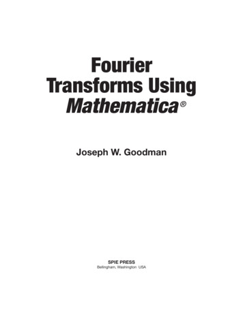
7If the filter function H is, say, the CTF, then the resulting spectrum will resemble the square of the CTF.This is illustrated in the figure below.Figure 1. Power spectra of random signals. Left column, functions of x; right column,functions of the frequency variable u. A, the basic random signal, consisting ofnormally-distributed random numbers. B, its power spectrum. The mean value of thepower spectrum is the same as the variance of the signal, 1 in this case. C, filterfunction—in this case, of the form of the defocus contrast-transfer function. D, theoriginal signal, but with the CTF applied. E, power spectrum of the filtered signal,with a smooth curve superimposed, computed as (𝑪𝑻𝑭)𝟐. Note that the powerspectrum has minima at the same frequency values as zeros in the CTF.AppendixCorrelationAn operation closely related to convolution is correlation, which is an operation that is often used tocompare the similarity of two functions. If we say that f(x) is the correlation 𝑔 ℎ we meanT𝑓(𝑥) BT 𝑔(𝑥 𝑠)ℎ(𝑠)𝑑𝑠.(A1)This is the same as taking one function g, shifting it by x, and then multiplying it by another function hand summing the product up. If g and h are the same except that they’re shifted relative to each other,then f(x) will have a maximum at the proper shift value. The correlation has a simple Fourier transformtoo.'(𝑔 ℎ ) 𝐺 𝐻 where the asterisk means complex conjugate. This can be derived from the fact that reflection maps tocomplex conjugation, i.e.'(𝑔( 𝑥) ) 𝐺 (𝑢)and the difference between the integrals in (12) and (A1) can be obtained if h is reflected.

Properties of the 1D Fourier transform Once you know a few transform pairs like the ones I outlined above, you can compute lots of FTs very simply using the following properties of transform pairs: 1. Linearit