WIXLIB

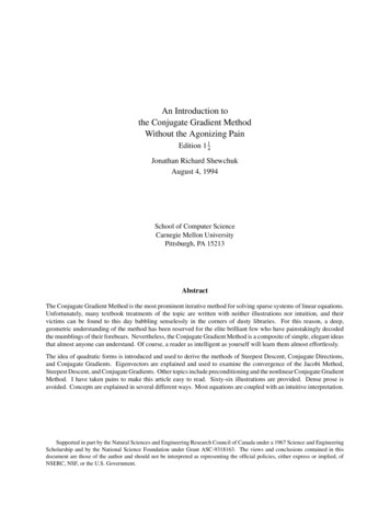
The Quadratic Form(a)(b); . 1 2; . 1 11(d); . 1 2 2(c) 5; . 1 21 1Figure 5: (a) Quadratic form for a positive-definite matrix. (b) For a negative-definite matrix. (c) For asingular (and positive-indefinite) matrix. A line that runs through the bottom of the valley is the set ofsolutions. (d) For an indefinite matrix. Because the solution is a saddle point, Steepest Descent and CGwill not work. In three dimensions or higher, a singular matrix can also have a saddle.; M1 f H ; 1 solution is a minimum of . , socan be solved by finding an that minimizes . . (If is not 6 G1g Y h . Note thatsymmetric, then Equation 6 hints that CG will find a solution to the system 21 .)6 G 11is symmetric.).2 )Why do symmetric positive-definite matrices have this nice property? Consider the relationship between W 8 1 . From Equation 3 one can show (Appendix C1)at some arbitrary point i and at the solution point that if is symmetric (be it positive-definite or not),; If ; .ji 1 ; . M1)1.ji2*Y 1 .ji *k M1 4 is positive-definite as well, then by Inequality 2, the latter term is positive for all iYl;is a global minimum of .(8). It follows that; M1The fact that . is a paraboloid is our best intuition of what it means for a matrix to be positive-definite. If is not positive-definite, there are several other possibilities. could be negative-definite — the result of negating a positive-definite matrix (see Figure 2, but hold it upside-down). might be singular, in which; case no solution is unique; the set of solutions is a line or hyperplane having a uniform value for . If is none of the above, then is a saddle point, and techniques like Steepest Descent and CG will likely fail.Figure 5 demonstrates the possibilities. The values of and @ determine where the minimum point of theparaboloid lies, but do not affect the paraboloid’s shape.Why go to the trouble of converting the linear system into a tougher-looking problem? The methodsunder study — Steepest Descent and CG — were developed and are intuitively understood in terms ofminimization problems like Figure 2, not in terms of intersecting hyperplanes such as Figure 1.

6Jonathan Richard Shewchuk4. The Method of Steepest Descent mIn the method of Steepest Descent, we start at an arbitrary point 0n and slide down to the bottom of the m m until we are satisfied that we are close enough to theparaboloid. We take a series of steps 1 n E 2n Esolution .;When we take a step, we choose the direction in which decreases most quickly, which is the direction* ; ] . m " 1U o*Y m " .;] m 1opposite . " n . According to Equation 7, this direction isnnm q m *A "nAllow me to introduce a few definitions, which you should memorize. The error p " nis a s*t mm""vector that indicates how far we are from the solution. The residual r nindicateshowfarwenmu * m""are from the correct value of . It is easy to see that r nasp n , and you shouldm think v* ;of] . the m " residual1 , and youbeing the error transformed by into the same space as . More importantly, r " nnshould also think of the residual as the direction of steepest descent. For nonlinear problems, discussed inSection 14, only the latter definition applies. So remember, whenever you read “residual”, think “directionof steepest descent.” m wJx**Suppose we start at 0 n2 2L . Our first step, along the direction of steepest descent, will fallEsomewhere on the solid line in Figure 6(a). In other words, we will choose a point m 4 mm1n0 n )Ay r 0 nThe question is, how big a step should we take?(9);A line search is a procedure that chooses y to minimize along a line. Figure 6(b) illustrates this task:we are restricted to choosing a point on the intersection of the vertical plane and the paraboloid. Figure 6(c)is the parabola defined by the intersection of these surfaces. What is the value of y at the base of theparabola?; m 1;From basic calculus, y minimizes when the directional derivative z . 1n is equal to zero. By the; m 16 ; ] . m 1 z m ; ] . m 1 r m . Setting this expressionz {chain rule, z . 1nto zero, we find that y1n ;1 n11n0nm m]z { so that r 0n and z . { 1n are orthogonal (see Figure 6(d)).should be chosenThere is an intuitive reason why we should expect these vectors to be orthogonal at the minimum.Figure 7 shows the gradient vectors at various points along the search line. The slope of the parabola(Figure 6(c)) at any point is equal to the magnitude of the projection of the gradient onto the line (Figure 7,;;dotted arrows). These projections represent the rate of increase of as one traverses the search line. isminimized where the projection is zero — where the gradient is orthogonal to the search line.; ] . ( m 1 * r m , and we have1n1nr m 1 n r m 0 n . s*Y m 1n 1 r m 0n . o*Y . m 0n )Ay r m 0n 1}1 r m 0n . s*Y m 0n 1 r m 0n * y . r m 0n 1 r m 0n . s*Y m 0n 1 r m 0n r m 0 n r m 0 n To determine y , note thaty000 0 m 1 my . r 0n r 0nm m 1y r 0n . r 0nr m 0 n r m 0nr m 0n r m 0n

The Method of Steepest Descent27(a)(b)42 m-40n-2 p m 0n2-2 461501005001 2.5 02-4-2.5-5-6m 1; . m"n )Ay r " n(c) -2.502; . M 1 2.5 51(d)4140120100806040202-4 m-2-21n4261-4y0.2 0.4 0.6 -6Figure 6: The method of Steepest Descent. (a) Starting at j 2 2 , take a step in the direction of steepestNNdescent of . (b) Find the point on the intersection of these two surfaces that minimizes . (c) This parabolais the intersection of surfaces. The bottommost point is our target. (d) The gradient at the bottommost pointis orthogonal to the gradient of the previous step. 221 -2-11231-1-2-3Figure 7: The gradient NZ[ is shown at several locations along the search line (solid arrows). Each gradient’sprojection onto the line is also shown (dotted arrows). The gradient vectors represent the direction ofsteepest increase of , and the projections represent the rate of increase as one traverses the search line.On the search line, is minimized where the gradient is orthogonal to the search line.NN

Jonathan Richard Shewchuk8242 -2-4 m0n2-2461 -4-6Figure 8: Here, the method of Steepest Descent starts at j 2 2 9 2 and converges at 2.Putting it all together, the method of Steepest Descent is:r m " n U*? (m " n Emm " r m " n r " m ny n r m" r "n E (m " % (m " n m " r m "n )Ay n n1n(10)(11)(12)The example is run until it converges in Figure 8. Note the zigzag path, which appears because eachgradient is orthogonal to the previous gradient.The algorithm, as written above, requires two matrix-vector multiplications per iteration. The computational cost of Steepest Descent is dominated by matrix-vector products; fortunately, one can be eliminated.* and adding , we haveBy premultiplying both sides of Equation 12 byr m " 1n r m " n * y m " n r m " n(13)mAlthough Equation 10 is still needed to compute r 0 n , Equation 13 can be used for every iteration thereafter. The product r , which occurs in both Equations 11 and 13, need only be computed once. The disadvantageof using this recurrence is that the sequence defined by Equation 13 is generated without any feedback from m mthe value of " n , so that accumulation of floating point roundoff error may cause " n to converge to some point near . This effect can be avoided by periodically using Equation 10 to recompute the correct residual.Before analyzing the convergence of Steepest Descent, I must digress to ensure that you have a solidunderstanding of eigenvectors.

Thinking with Eigenvectors and Eigenvalues5. Thinking with Eigenvectors and Eigenvalues9After my one course in linear algebra, I knew eigenvectors and eigenvalues like the back of my head. If yourinstructor was anything like mine, you recall solving problems involving eigendoohickeys, but you neverreally understood them. Unfortunately, without an intuitive grasp of them, CG won’t make sense either. Ifyou’re already eigentalented, feel free to skip this section.Eigenvectors are used primarily as an analysis tool; Steepest Descent and CG do not calculate the valueof any eigenvectors as part of the algorithm1 .5.1. Eigen do it if I try//An eigenvector of a matrix is a nonzero vector that does not rotate when is applied to it (exceptperhaps to point in precisely the opposite direction). may change length or reverse its direction, but it/ . The value iswon’t turn sideways. In other words, there is some scalar constant such that /an eigenvalue of . For any constant y , the vector y is also an eigenvector with eigenvalue , because/ . 1c / . In other words, if you scale an eigenvector, it’s still an eigenvector.yyy/Why should you care? Iterative methods often depend on applying to a vector over and over" again."// When is repeatedly applied to an eigenvector , one of two thingscan happen. If S 1, then ", 1, then / will grow to infinity (Figure 10). Each will vanish as approaches infinity (Figure 9). If /time is applied, the vector grows or shrinks according to the value of . B2 vv B3 vBvFigure 9: is an eigenvector of with a corresponding eigenvalue of 0 5. As increases, \ convergesto zero.vBv B2 v B3 vFigure 10: Here, has a corresponding eigenvalue of 2. As increases, Q diverges to infinity.1However, there are practical applications for eigenvectors. The eigenvectors of the stiffness matrix associated with a discretizedstructure of uniform density represent the natural modes of vibration of the structure being studied. For instance, the eigenvectorsof the stiffness matrix associated with a one-dimensional uniformly-spaced mesh are sine waves, and to express vibrations as alinear combination of these eigenvectors is equivalent to performing a discrete Fourier transform.

/IfJonathan Richard Shewchukis symmetric (and often if it is not), then there exists a set of linearly independent eigenvectors/of , denoted 1 2 . This set is not unique, because each eigenvector can be scaled by an arbitraryE E Enonzero constant. Each eigenvector has a corresponding eigenvalue, denoted 1 2 . These areE E Euniquely defined for a given matrix. The eigenvalues may or may not be equal to each other; for instance,the eigenvalues of the identity matrix are all one, and every nonzero vector is an eigenvector of .10/What if is applied to a vector that is not an eigenvector? A very important skill in understandinglinear algebra — the skill this section is written to teach — is to think of a vector as a sum of other vectors" forms a basis for (because awhose behavior is understood. Consider that the set of eigenvectors a /symmetric has eigenvectors that are linearly independent). Any -dimensional vector can be expressedas a linear combination of these eigenvectors, and because matrix-vector multiplication is distributive, one/can examine the effect of on each eigenvector separately. / In Figure 11, a vector is illustrated as a sum of two eigenvectors 1 and 2 . Applyingto is/equivalentthe " eigenvectors, and summing the result. On repeated application, we" have/ " 4/ " to applying/ " " to/ willthan one, 1)21 1 ) 2 2 . If the magnitudes of all the eigenvalues are smaller/converge to zero, because the eigenvectors that compose converge to zero when is repeatedly applied. If one of the eigenvalues has magnitude greater than one, will diverge to infinity. This is why numericalanalysts attach importance to the spectral radius of a matrix:/ 1 . " " is an eigenvalue of / . E /1 If we want to converge to zero quickly, .should be less than one, and preferably as small as possible.max v 2v1B3 xBx B2 xxFigure 11: The vectorP(solid arrow) can be expressed as a linear combination of eigenvectors (dashedarrows), whose associated eigenvalues are 1 0 7 and 22. The effect of repeatedly applying tois best understood by examining the effect of on each eigenvector. When is repeatedly applied, oneeigenvector converges to zero while the other diverges; hence,also diverges. V VA \P PIt’s important to mention that there is a family of nonsymmetric matrices that do not have a full set ofindependent eigenvectors. These matrices are known as defective, a name that betrays the well-deservedhostility they have earned from frustrated linear algebraists. The details are too complicated to describe inthis article, but the behavior of defective matricescan be analyzed in terms of generalized eigenvectors and/ " convergesgeneralized eigenvalues. The rule thatto zero if and only if all the generalized eigenvalueshave magnitude smaller than one still holds, but is harder to prove.Here’s a useful fact: the eigenvalues of a positive-definite matrix are all positive. This fact can be provenfrom the definition of eigenvalue:/ / (/ is positive (for nonzero By the definition of positive-definite, the ). Hence, must be positive also.

Thinking with Eigenvectors and Eigenvalues115.2. Jacobi iterationsOf course, a procedure that always converges to zero isn’t going to help you attract friends. Consider a more 3 u . The matrix is split into two parts: , whoseuseful procedure: the Jacobi Method for solving diagonal elements are identical to those of , and whose off-diagonal elements are zero; and , whose .diagonal elements are zero, and whose off-diagonal elements are identical to those of . Thus,)We derive the Jacobi Method: * * 8 1) 8)/W )A E1where/ * 8 1 E 81(14)Because is diagonal, it is easy to invert. This identity can be converted into an iterative method byforming the recurrence m " /5 (m "(15)n )¡ 1n mGiven a starting vector 0 n , this formula generates a sequence of vectors. Our hope is that each successive vector will be closer to the solution than the last. is called a stationary point of Equation 15, because if m " % , then m " will also equal .1nnNow, this derivation may seem quite arbitrary to you, and you’re right. We could have formed any number of identities for instead of Equation 14. In fact, simply by splitting differently — that is,by choosing a different and — we could have derived the Gauss-Seidel method, or the method of/Successive Over-Relaxation (SOR). Our hope is that we have chosen a splitting for which has a smallspectral radius. Here, I chose the Jacobi splitting arbitrarily for simplicity. Suppose we start with some arbitrary vectorto the result. What does each iteration do? m0n . For each iteration, we apply/to this vector, then addAgain, apply the principle of thinking of a vector as a sum of other, well-understood vectors. Express m meach iterate " n as the sum of the exact solution and the error term p " n . Then, Equation 15 becomes m " 1n /W m "/ . n )Ap m " 1) m /W ) n / ¡p "n )A/ p m )"(by Equation 14))nE p m " 1n / p m " n(16) m Each iteration does not affect the “correct part” of " n (because is a stationary point); but each iteration/ 1 1, then the error term p m " willdoes affect the error term. It is apparent from Equation 16 that if .n mconverge to zero as approaches infinity. Hence, the initial vector 0 n has no effect on the inevitableoutcome! (m Of course, the choice of 0 n does affect the number of iterations required to converge to within/ 1a given tolerance. However, its effect is less important than that of the spectral radius . , which/determines the speed of convergence. Suppose that a is the eigenvector of with the largest eigenvalue/ 1 ). If the initial error p m , expressed as a linear combination of eigenvectors, includes a(so that .0ncomponent in the direction of , this component will be the slowest to converge.

Jonathan Richard Shewchuk12242 -2-424617-22-4-6Figure 12: The eigenvectors ofTare directed along the axes of the paraboloid defined by the quadraticform. Each eigenvector is labeled with its associated eigenvalue. Each eigenvalue is proportional tothe steepness of the corresponding slope.N OQPSR/ is not generally symmetric (even if is), and may even be defective. However, the rate of convergence/71 of the Jacobi Method depends largely on . , which depends on . Unfortunately, Jacobi does not converge for every , or even for every positive-definite .5.3. A Concrete ExampleTo demonstrate these ideas, I shall solve the system specified by Equation 4. First, we need a method offinding eigenvalues and eigenvectors. By definition, for any eigenvector with eigenvalue ,Eigenvectors are nonzero, so *Y ' .§ ' *YG 1 0must be singular. Then,det .§ ' *? G1c 0* The determinant of is called the characteristic polynomial. It is a degree polynomial in whose roots are the set of eigenvalues. The characteristic polynomial of (from Equation 4) is* 3 * 2 *B * 2 * 6 D 2 9 )det .§ * 71 §. * 21E and the eigenvalues are 7 and 2. To find the eigenvector associated with 7,* 2 B Y*G 1C B4* 2 1 D 1D 0.§ 2 4 1 * 2 2 014

Convergence Analysis of Steepest Descent13 JxJ*Any solution to this equation is an eigenvector; say, 1 2L . By the same method, we find that 2 1LEEis an eigenvector corresponding to the eigenvalue 2. In Figure 12, we see that these eigenvectors coincidewith the axes of the familiar ellipsoid, and that a larger eigenvalue corresponds to a steeper slope. (Negative;eigenvalues indicate that decreases along the axis, as in Figures 5(b) and 5(d).)Now, let’s see the Jacobi Method in action. Using the constants specified by Equation 4, we have m " 1n * B m" BDD n)* 2 m B 2" n ) * 3430 D3 D13016B *013/Jj B00 22 0130016* B *28 DDJx* The eigenvectors ofare 2 1L with eigenvalue2 ª 3, and2 1L with eigenvalue 2 ª 3. EEThese are graphed in Figure 13(a); note that they do not coincide with the eigenvectors of , and are notrelated to the axes of the paraboloid.Figure 13(b) shows the convergence of the Jacobi method. The mysterious path the algorithm takes canbe understood by watching the eigenvector components of each successive error term (Figures 13(c), (d),and (e)). Figure 13(f) plots the eigenvector components as arrowheads. These are converging normally atthe rate defined by their eigenvalues, as in Figure 11.I hope that this section has convinced you that eigenvectors are useful tools, and not just bizarre torturedevices inflicted on you by your professors for the

1. Introduction 1 2. Notation 1 3. The Quadratic Form 2 4. The Method of Steepest Descent 6 5. Thinking with Eigenvectors and Eigenvalues 9 5.1. Eigen do it if I try 9 5.2. Jacobi iterations 11 5.3. A Concrete Example 12 6. Convergence Analysis of Steepest Descent 13 6.1. Instant Results 13 6.2. General Convergence 17 7. The Method of Conjugate .