Transcription
The Mandelbrot SetThe Mandelbrot set, the topic of this notebook, became famous as a simple model which produces extraordinarilycomplicated (and "beautiful") fractal structures. It is defined as the set of all points in the complex plane, (cx , cy ) suchthat the complex mapz Ø z2 ci.e. zn 1 zn 2 c, does not escape to infinity starting from z 0. As we shall see it is related to the logistic map, and canbe thought of as a generalization of the logistic map to the complex plane.The code below is used to generate a Mandelbrot set. It takes as arguments the real and imaginary parts (cx, cy) ofthe complex number c, and returns (minus) the number of iterations that the map takes to escape (in practice to get to z 2, because one can show that a point will escape to infinity if it once gets to a value where z 2) up to a maximum of lim. Note the use of the While command (a similar programming style to that used in C).In[1]: Clear@"Global *"DIn[2]: mandelbrot@cx , cy , lim D : Hz 0; ct 0;While @ Abs@zD 2.0 && ct lim,z z 2 cx I cy; ctD;- ctL;For example,In[3]: Out[3] mandelbrot@0.5, 0.5, 50D-5so starting from c 0.5 0.5 I, it takes 5 iterations for the point z 0 to escape to z 2.Next we write the function as a module, rather than just a function, so that local variables, ct, and z, can be defined inthe routine independentally of whether any variables of the same name exist in the rest of the Mathematica session.Note that the local variables can be initialized at the same time as they are declared, and we do this here:In[6]: Clear@mandelbrotD;mandelbrot@cx , cy , lim D : Module @ 8 z 0, ct 0 ,While @ Abs@zD 2.0 && ct lim,z z 2 cx I cy; ctD;- ctD;This routine is quite slow. Next we compile it so that it runs faster. To compile a function f[x ] x Log[x] andcall the compiled version fc, we write fc Compile[{x}, x Log[x] ], where the quantity(ies) in curlybrackets is (are) the argument(s). (The notation is similar to that for a pure function, for which we could write f Function[{x}, x log[x] ]). The following function is the compiled version of the above Module:
2mandelbrot.nbIn[8]: mandelbrotC Compile @ 8 cx, cy, lim ,Module@ 8 z 0. I 0., ct 0 ,While @ Abs@zD 2.0 && ct lim,z z 2 cx I cy; ctD;- ctDD;Note that the arguments appear on the RHS of the function definition, rather than on the LHS as in the uncompiledversion.Below we use show the whole of the Mandelbrot set with a coarse resolution and compare the timing of the compiledand uncompiled version. The value of the function being plotted is characterized by the degree of blackness in aDensityPlot. The smaller the number the blacker it is. Since we compute the negative of the number of iterations, theblackest region is where the number of iterations is greatest.In[9]: Out[9] In[10]: Out[10] Timing@DensityPlot@mandelbrot@x, y, 100D, 8x, - 2, 0.6 , 8y, - 1.3, 1.3 , PlotPoints Ø 40,Mesh Ø False, ColorFunction Ø GrayLevel, Epilog Ø 88GrayLevel@0.6D, Thickness@0.008D,Line@88- 0.3, 0.6 , 8- 0.3, 1 , 80.1, 1 , 80.1, 0.6 , 8- 0.3, 0.6 D DD:0.901516, Timing@DensityPlot@mandelbrotC@x, y, 100D, 8x, - 2, 0.6 , 8y, - 1.3, 1.3 , PlotPoints Ø 40,Mesh Ø False, ColorFunction Ø GrayLevel, Epilog Ø 88GrayLevel@0.6D, Thickness@0.008D,Line@88- 0.3, 0.6 , 8- 0.3, 1 , 80.1, 1 , 80.1, 0.6 , 8- 0.3, 0.6 D DD:0.176187, Note that the compiled version is about 5 times faster.Remember that the darker the region the more iterations were needed to escape.Now we use the compiled version to show the set with finer resolution and in color, using the ColorFunction option ofDensityPlot. The way we call the Hue function is an example of a Mathematica "pure function". Areas in blue need alarge number of iterations to escape while those in red need rather few. (Note that I plotted minus the result of themandelbrotC function.)
mandelbrot.nbIn[11]: 3DensityPlotA- mandelbrotC@x, y, 200D, 8x, - 2, 0.6 , 8y, - 1.3, 1.3 ,PlotPoints Ø 200, Mesh Ø False, ColorFunction Ø IHueA0.75 Ò10.6 E &M,Epilog Ø 88GrayLevel@0.6D, Thickness@0.008D,Line@88- 0.3, 0.6 , 8- 0.3, 1 , 80.1, 1 , 80.1, 0.6 , 8- 0.3, 0.6 D EOut[11] This is the famous Mandelbrot set. Even at this resolution it is amazingly complicated. However, the full depths of itscomplexity can only be appreciated when we blow up different regions of it, which we will do shortly.Notice that the largest part of the figure is in the shape of a cardioid out of which grow many "buds" of different sizes.The largest bud, to the left of the cardioid joins it at one point, x -3/4, y 0. The "cusp" in the cardoid on the right isat x 1/4, y 0. Clearly if c is real then, since we start off with z real Hz0 0), all subsequent values zn must also bereal. There is actually a strong connection between the map used to generate the Mandelbrot set, zn 1 z2n c,specialized to real c (and z), and the logistic map xn 1 4 l xn H1 - xn L. To see this let zn a xn b and verify thatthe two maps are the same if b 2l and a -4l with c then related to l byc 2 l H1 - 2 lL .Hence, as l varies from 1/4 to 1 (all the interesting region of the logistic map except for the trivial part with a fixedpoint at x 0) c varies from 1/4 to -2. The fixed point region of the logistic map, 1/4 l 3/4 corresponds to 1/4 c -3/4, which is precisely the region of the big cardioid. The period two limit cycle, 3/4 l 0.8626 corresponds tothe largest bud the left of it, the period 4 limit cycle to the bud growing out to the left of that and so on. Additional"blobs" further to the left on the x axis, and which appear separated from the main region (though they are not)correspond to islands of limit cycle behavior in the logistic map, which, as you will recall, period double their way tochaos.There is therefore a connection between the Mandelbrot set and the logistic map. However, the full richness of theMandelbrot set is only seen by going into the complex plane.Now we will blow up different regions of the set, starting with an enlarged the bud at the top of the cardioid (the areain the grey box in the figure above)
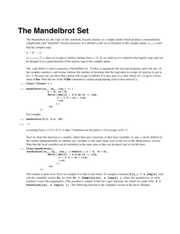
4mandelbrot.nbIn[12]: DensityPlotA- mandelbrotC@x, y, 200D, 8x, - 0.3, 0.1 , 8y, 0.6, 1 ,PlotPoints Ø 200, Mesh Ø False, ColorFunction Ø IHueA0.75 Ò10.63 E &M,Epilog Ø 88GrayLevel@0.6D, Thickness@0.008D, Line@88- 0.0234, 0.99875 , 8- 0.0234, 0.99925 ,8- 0.0229, 0.99925 , 8- 0.0229, 0.99875 , 8- 0.0234, 0.99875 D EOut[12] Notice how the same structure is repeated in many places and in many different scales. This is characteristic of afractal structure.Below we show a tiny region at the top edge in the above around x -0.023, y 1. (It is marked by a grey box in theabove figure but it is so small it is hard to see.) In order to bring out the details of the structure we have increased themaximum number of iterations to 500.
mandelbrot.nbIn[13]: DensityPlotAmandelbrotC@x, y, 1000D, 8x, - 0.0234, - 0.0229 , 8y, 0.99875, 0.99925 ,PlotPoints Ø 200, Mesh Ø False, ColorFunction Ø IHueA0.8 Ò17 E &MEOut[13] We find the Mandelbrot set again! Notice how expanded the scale is. This miniature Mandelbrot set is actuallyconnected to the rest of the set, but the connecting filaments are too fine to be seen on this plot.Next we look at a greatly enlarged view of the edge of the cardioid in the first high resolution figure (3rd figureoverall), in the notch near where it joins the bud at the left. The scale is nearly a thousand times greater than in thefirst figure.In[14]: Out[14] DensityPlot@- mandelbrotC@x, y, 1000D, 8x, - 0.75, - 0.747 , 8y, 0.06, 0.063 ,PlotPoints Ø 200, Mesh Ø False, ColorFunction Ø HHue@0.75 Ò1D &L,Epilog Ø 88GrayLevel@1.D, Thickness@0.008D, Line@88- 0.7488, 0.06055 , 8- 0.7488, 0.06075 ,8- 0.7486, 0.06075 , 8- 0.7486, 0.06055 , 8- 0.7488, 0.06055 D D5
6mandelbrot.nbNotice the complicated spiral structures.Suppose we now blow up the center of the spiral arm near the bottom and slightly to the left. What will be see?In[15]: DensityPlot@- mandelbrotC@x, y, 500D, 8x, - 0.7488, - 0.7486 , 8y, 0.06055, 0.06075 ,ColorFunction Ø HHue@0.7 Ò1D &L, PlotPoints Ø 200, Mesh Ø False, Epilog Ø88GrayLevel@1.D, Thickness@0.008D, Line@88- 0.74871, 0.06069 , 8- 0.74871, 0.06072 ,8- 0.74868, 0.06072 , 8- 0.74868, 0.06069 , 8- 0.74871, 0.06069 D DOut[15] There is an enormous amout of detail in the spiral arm.Let's continue to increase the scale and enlarge a section of the arm, at the highest point of the spiral.
mandelbrot.nbIn[16]: 7DensityPlot@mandelbrotC@x, y, 1000D, 8x, - 0.74871, - 0.74868 ,8y, 0.06069, 0.06072 , PlotPoints Ø 200, Mesh Ø False, ColorFunction Ø GrayLevel,FrameTicks Ø 88- 0.74871, - 0.7487, - 0.74869, - 0.74868 , Automatic, None, None , Epilog Ø88GrayLevel@1.D, Thickness@0.008D, Line@88- 0.748703, 0.0607 , 8- 0.748703, 0.060702 ,8- 0.748701, 0.060702 , 8- 0.748701, 0.0607 , 8- 0.748703, 0.0607 D DOut[16] We have now blown up the figure of the entire Mandelbrot set at the top by a factor of about 105 and we see intricatedetails down to the smallest scale visible.Next let's blow up one of the two regions where a thin loopy strand splits into two spirals turning in opposite directions. We take the one near x -0.748702, y 0.060701.
8mandelbrot.nbIn[17]: DensityPlot@mandelbrotC@x, y, 1000D, 8x, - 0.748703, - 0.748701 ,8y, 0.0607, 0.060702 , PlotPoints Ø 200, Mesh Ø False,ColorFunction Ø GrayLevel, Epilog Ø 88GrayLevel@1.D, Thickness@0.008D,Line@88- 0.7487023, 0.06070105 , 8- 0.7487023, 0.06070125 ,8- 0.7487021, 0.06070125 , 8- 0.7487021, 0.06070105 , 8- 0.7487023, 0.06070105 D DOut[17] Finally we zoom in on the "blob" at the center of the figure (surrounded by 4 spirals).In[18]: DensityPlot@- mandelbrotC@x, y, 2000D,8x, - 0.7487023, - 0.7487021 , 8y, 0.06070105, 0.06070125 ,ColorFunction Ø HHue@0.75 Ò1D &L, PlotPoints Ø 100, Mesh Ø False,FrameTicks Ø 88- 0.7487023, - 0.7487022, - 0.7487021 , 80.0607011, 0.0607012 , None, None DOut[18] Lo and behold, the Mandelbrot set again! Note that the scale of this figure is about 107 times greater than in the firstfigure we showed of the Mandelbrot set.
mandelbrot.nb9Julia SetThe Julia set is related to the Mandelbrot, set since it also involves the study of the escape to infinity of a map, z - f(z)involving a parameter c, but rather than fixing the initial point to be z 0 and considering the set of all values of c forwhich z does not escape to infinity, we now consider the set of all initial points z that does not not escape to infinity fora fixed complex c. The form of the Julia set depends very much on the choice of the function f(z) and the parameter c.The code below iterates the quadratic map, z - z 2 c, the same as for the Mandelbrot set, and determines thenumber of iterations it takes for z to escape for the given initial value of z ( x iy) and the (fixed) value of c ( cx icy).In[19]: juliaC Compile @ 8 x, y, lim, cx, cy ,Module@ 8 z, ct 0 ,z x I y;While@ Abs@zD 2.0 && ct lim,z z 2 Hcx I cyL; ctD;ctDD;The plot below show the Julia set for a particular value of c.In[20]: DensityPlot@- juliaC@x, y, 200, 0.27334, 0.00742D, 8x, - 1.5, 1.5 ,8y, - 1.5, 1.5 , ColorFunction Ø HHue@0.55 Ò1D &L, PlotPoints Ø 200, Mesh Ø FalseDOut[20] We now show the central region of the above plot enlarged.
10mandelbrot.nbIn[21]: Out[21] DensityPlot@- juliaC@x, y, 50, 0.27334, 0.00742D, 8x, - 0.5, 0.5 ,8y, - 0.5, 0.5 , PlotPoints Ø 200, ColorFunction Ø HHue@0.75 Ò1D &L, Mesh Ø FalseD
Notice that the largest part of the figure is in the shape of a cardioid out of which grow many "buds" of different sizes. . -3/4, which is precisely the region of the big cardioid. The period two limit cycle, 3/4 l 0.8626 corresponds to the largest bud the left of it, the period 4 limit cycle to the bud growing out to the left of that .