WIXLIB

Predictive dynamics: an optimization-based novel approach for human motion simulationq f –1 (τ , t)qFig. 3 Constraints for a bio-systemqτ f (q, t)Fig. 1 Flowcharts a forward dynamics and b inverse dynamicsnumerical integration. The optimization problem is usuallya large-scale nonlinear programming problem with manydesign variables and constraints. To solve the problem efficiently, modern optimization methods that take advantageof the structure of the problem need to be used.The studied bio-system is represented as S and the corresponding mathematical model as M . The general equationsof motion for the model M are written as: f q, q̇, q̈, t τaccuracy. However, the boundary conditions and some stateresponse of the system might be available. In this case, neither forward dynamics nor inverse dynamics can be appliedto the bio-system S directly. As a consequence, the predictive dynamics procedure is proposed to solve these typesof problems. The basic idea is to formulate a nonlinearoptimization problem based on the physics of motion (thedynamics of the motion). An appropriate performance measure (objective function) for the bio-system is defined andminimized subject to the available information about thesystem that imposes various constraints. Thus the predictive dynamics approach is formulated for the system M asfollows:minJ (q, τ , t)s.t. :τ f (q, t) 0q,τg (ϒ) 0(1)(2)q q qLwhere q, q̇, q̈ R N are the state variables, and τ R N arethe generalized forces. This dynamics problem is definedover the time domain (T0 , T ) with boundary ·{T0 , T } , t , t being the time and the symbol (·) indicating derivative with respect to t. The superscript N representsthe number of DOF of model M .Forward dynamics calculates the motion (q, q̇, and q̈)from the force τ by integrating (1) with the specified initial conditions. In contrast, inverse dynamics computes theassociated force τ that leads to a prescribed motion for thesystem. The two procedures are depicted in Fig. 1. Forsimplicity, we use only q to represent kinematics of thesystem.In practice, it is difficult to measure complete displacement (q) and force (τ ) histories accurately for a bio-systemwith many DOFs, especially involving a complex motion.This is because the experimental measurement is either notaccurate enough or too expensive to achieve the requiredUτ L τ τUwhere g are the constraints defined based on the availableinformation ϒ about the system S. q and τ are subjectto their lower and upper bounds, respectively. For thebio-system, the objective function is usually called the performance measure. The flowchart of predictive dynamics isshown in Fig. 2.Two challenging problems arise naturally for the predictive dynamics approach: (1) the functional form of theperformance measure is unknown; and (2) the constraintsare undetermined. Before turning to these two importantissues, the evaluation criterion for predictive dynamics isfirst proposed, i.e., how to validate the predictive dynamicssolution of model M with that of the real system S.Table 1 Four cases of swing motion examined by predictive dynamicsMotionCaseAvailable informationSimple swing without1Boundary conditions2Boundary conditions3Boundary conditions andoscillationOscillating motionresponse at one time point4Boundary conditions andresponse at two time pointsFig. 2 Flowchart of predictive dynamics

Y. Xiang et al.Fig. 4 Single pendulumyoτxqlchosen as determinants to define a specific motion such aswalking and running. For walking motion, the six determinants correspond to the lower extremities and pelvic motion(Saunders et al. 1953). Therefore, instead of using all thejoint angle and torque profiles in (3), only the determinantand torque profiles may be used in (3) to validate the task.Furthermore, the predictive dynamics structure has veryflexible optimization formulation in terms of constraints andperformance measures for dynamic human motion prediction. For instance, the constraints allow one to model theboundary conditions and state response of the problem, andthe performance measure allows one to study what driveshuman motion. However, this assumes that the performancemeasure represents a physically significant quantity, not justa curve fit to predetermined data. Therefore, once the simulation model is validated, it can be used to show causeand effect, study an injury problem, analyze pathologicalmotion, and so on.mgSuppose q and τ represent the natural motion of thebio-system S. One way to quantify the accuracy of the predictive dynamics solution for the bio-system is to evaluatethe percentage error of the residuals of the predicted forceand displacement histories using a norm, as follows: T q̄ q τ̄ τ dt0ε T q τ dt(3)0where q̄ and τ̄ are optimal values obtained from the predictive dynamics in (2); T is the total time.For human motion validation, some well studiedkinematics variables (angles and displacements) have beenFig. 5 Forward dynamicssolved by ADAMS3 Performance measuresThe unknown performance measure needs to be identifiedfirst. Two basic methods are available: one is the trialand-error method, and the other is the inferring method,which requires more insight into the physical process of thebio-system.3.1 Trial-and-errorThe trial-and-error method enumerates the hypothesizedperformance function J to solve the predictive dynamicsproblem in (2). Then the error in (3) is checked with thereal solution that is obtained from either the exact analytical

Predictive dynamics: an optimization-based novel approach for human motion simulation0-5Joint velocity (rad/s)solution or an experiment with sufficiently small error. Oncethe error is in an acceptable small range, the correspondingfunction J is treated as the performance measure for predictive dynamics. However, this is a trial-and-error process,with no guarantee of success.In practice, the performance set includes many differentkinematics and dynamics criteria such as time minimization,effort minimization, energy minimization, jerk minimization, and so on. However, a performance measure that iswell studied in the biomechanics literature is often used tonarrow down the trial-and-error process; for example, minimizing the squares of all actuating torques or minimizingthe maximum torque for all joints.-10-15Torque squareConstantMin-maxMinimum timeForward dynamics-20-25-300.03.2 Inner optimization0.10.20.30.4Time (s)An alternative way to detect the performance measure isto use the inner optimization (nested optimization) method.The basic idea is to construct a local search space ofcost functions S J with a specific functional form basedon some insight into the physical processes governing thebio-system.SJ q, τ , t p J (q, τ , t)(4)where p is the parameter vector that needs to bedetermined.For instance, a performance measure for the bio-systemhas been identified as the sum of squares of all joint torqueswith coefficients p as in (5).S J (q, τ , t p ) T nτ0pi τi2 dt(5)i 10.0Joint angle (rad)wherenτ pi 1 and pi 0(6)i 1The parameters p are determined by solving the inneroptimization problem as defined in (7) so that the exactperformance measure can be identified.minpεs.t. : h (p) 0min S J (q, τ , t p )q,τs.t. : τ f (q, t) 0g(ϒ) 0q L q qUτ L τ τU(7)where h(p) 0 are the possible equality or inequality constraints on the parameters p satisfying the normalization andnon-negativity conditions. ε is the error defined in (3). Theprocess of identifying the unknown performance measure istransformed to find the parameters p that will minimize theerror ε.-0.5-1.0-1.5Torque squareConstantMin-maxMinimum timeForward dynamics-2.0-2.50.0Fig. 7 Joint velocity prediction of the single pendulum, Case 10.10.20.3Time (s)Fig. 6 Joint angle prediction of the single pendulum, Case 14 Constraints0.4Constraints are formulated based on the available information ϒ about the bio-system. In general, two types of constraints are included in this set: (a) boundary conditions, and(b) available state response at some time points q t j , t j , obtained from either experiments or observations. In

Y. Xiang et al.0.12The solution of (8) implies that the output set (q f , τ f )satisfies all linear and nonlinear constraints, but does notoptimize any performance measure for the bio-system. Thisis a feasible solution of the predictive dynamics problem.There are two purposes of obtaining a feasible solution forthe system: one is to test the feasibility of all the constraints,and the other is to get a solution that might be used as a goodinitial guess for the predictive dynamics with a physicalperformance measure.0.100.08Joint torque (Nm)0.060.040.020.00Torque squareMin-maxForward dynamics-0.02-0.04-0.064.2 Minimal set of constraints-0.08-0.100.00.10.20.30.40.5Time (s)Fig. 8 Joint torque prediction of the single pendulum, Case 1addition, boundary conditions consist ofboundary timeqt j , t j , and geometrical boundary X qt j , t j ,where X represents the global Cartesian coordinates thatcapture the geometrical environment for the bio-system. Forexample, given initial and final postures, a walking taskis performed to predict the walking motion between thetwo postures. The initial and final postures are the timeboundaries, and the ground is formulated as a geometrical boundary. However, there are many options for stateresponse constraints based on available information aboutthe walking motion, such as transition posture between single support and double support phases, knee flexion angleat mid-swing time point, etc. The overall set of constraintsis depicted in Fig. 3.It is obvious that the more information about the bio-systemis available, the more accurate the predictive dynamics solution is. As an extreme case, all the displacement and forcehistories can be available in the time domain . However, in most cases, only minimal information about thebio-system is available so that predictive dynamics seeksfor the minimal constraint set g (ϒminimal ) and an appropriate performance measure to simulate the applied force andresponse histories for the bio-system, as follows:J (q, τ ,t)minq,τs.t. : τ f (q, t) 0g (ϒminimal ) 0q L q qUτ L τ τU(9)The minimal constraint set depends on the complexity ofthe bio-system and the motion to be simulated. For a1.04.1 Feasible set0.5minq,τJ (q, τ , t) cs.t. : τ f (q, t) 0g(ϒ) 0q L q qUτ L τ τUwhere c is a constant.Torque squareMin-maxForward dynamics0.0Joint angle (rad)The feasible set of solutions for the problem is an importantissue for predictive dynamics. An infeasible set will resultin a null solution space for the system. This situation shouldalways be avoided while formulating a predictive dynamicsproblem. For a bio-system, feasibility of all the constraintscan be tested by solving the predictive dynamics problemwith a constant objective function as 1.01.21.41.61.8Time (s)Fig. 9 Joint angle prediction of the single pendulum, Case 22.0

Predictive dynamics: an optimization-based novel approach for human motion simulation1.61.41.2Joint torque (Nm)simple motion, boundary conditions alone might be enoughto reveal the entire motion; in this case, the minimal constraint set includes only boundary conditions. In contrast,for a complex motion, some state responses between theboundaries need to be known to simulate the real motion.Therefore, these state responses have to be included in theminimal constraint set.Torque squareMin-maxForward dynamics1.00.80.60.40.25 Discretization and scaling0.0-0.2The predictive dynamics problem in (2) is actually an optimal control problem with boundary conditions and somestate constraints. The classical method to solve the optimal control problem is to derive the optimality conditionfor the continuous variable optimization problem. However, beyond boundary conditions, the continuous methodhas difficulty dealing with discrete state constraints. Themost efficient way to solve a complex optimal control problem is to use nonlinear optimization techniques. The basicidea is to discretize the governing equations of motionusing a suitable numerical method and define finite dimensional approximation for the state and control variables.This process transforms the system differential equationsinto algebraic equations with parametric representation ofthe state and control variables. The performance measuresand the constraints are also evaluated in terms of discretestate and control values. Therefore, the original optimalcontrol problem is transformed into a nonlinear programming (NLP) problem.8Torque squareMin-maxForward dynamicsJoint velocity .0Time (s)Fig. 11 Joint torque prediction of the single pendulum, Case 2The time domain is first discretized into n intervals withstep size h i , as follows:0 t0 t1 · · · tn 1 tn T and h i ti 1 ti(10)The discretized state qh and force τ h can be expressed interms of interpolating functions and discrete nodal degreesof freedom (control points) Pq and Pτ . qh q Pq , h ;τ h τ (Pτ , h)(11)Thus, the discretized predictive dynamics problem is formulated as: min J qh , τ h , thq,τ s.t. : τ h f qh , th 0(12)g(ϒh ) 0LUq qh qτ L τh τUIn general, all the unknowns and the equations of motionshould be scaled to improve the numerical performance ofthe nonlinear optimization solver. Appropriate scale factorss are chosen so as to obtain quantities that have the samemagnitude order O (1). It is noted that scaling of a constraintdoes not change the constraint boundary, so it has no effecton the optimum solution.-6-8 J s q qh , s τ τ h , s t th s.t. : s τ τ h f s q qh , s t th 0g (ϒh ) 0s q q L s q qh s q qUsτ τ L sτ τ h sτ τ Uminq,τ-100.00.20.40.60.81.01.21.41.61.8Time (s)Fig. 10 Joint velocity prediction of the single pendulum, Case 22.0(13)

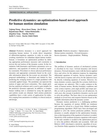
Y. Xiang et al.6 Numerical example: single pendulum8lI q̈ mg cos q Time (s)Fig. 13 Joint velocity prediction of the single pendulum, Case 3(14)where I is the moment of inertia, m is the mass, l is thelength, q is the joint angle, and τ is the external torque.The external torque is assumed to be a sinusoidal functiongiven as(Nm)(15)The geometrical and physical parameters of the rigid bar aretaken as I 0.0267 kg m2 , m 0.5 kg, and l 0.4 m. Withthe initial condition q(0) 0 and q̇ (0) 0, the forwarddynamics is solved by the ADAMS Runge–Kutta solver, asshown in Fig. 5, which is considered the true solution of thesystem.1.06.2 Simple swing motion with boundary conditionsThe swinging motion without oscillation is studied withthe initial and final conditions. The total time is randomlyselected as T 0.43 s (less than first half period of oscillation), and the single pendulum starts at rest in the horizontalposition and ends up with the final conditions that areobtained from Fig. 5 as q(T ) 2.40 rad and q̇ (T ) 5.86 rad/s. The swinging motion is driven by the externaltorque and gravity. Besides boundary condition and totaltravel time T , neither external torque nor joint angle isknown. Therefore, the predictive dynamics problem is formulated as in (16) to reveal the natural swing motion of thesingle pendulum.J (q, τ, t)lSubject to I q̈ mg cos q τ2q (0) 0, q̇ (0) 0q (T ) 2.40, q̇ (T ) 5.86, T 0.43 π q π 10 τ 10Minimize0.5Torque squareMin-maxForward dynamics0.0Joint angle (rad)Joint velocity (rad/s)The natural swinging motion of a single pendulum subjectedto external torque is considered. The swinging motion isfirst treated as a forward dynamics problem with the knownexternal force and solved by the multi-body dynamics solverADAMS. The solution is assumed to be the true responseof the system used to evaluate the results obtained withthe predictive dynamics formulation. Predictive dynamicsis implemented based on the available information about thesystem. Four cases are examined with predictive dynamicsas listed in Table 1.The pendulum pivots at the point O as shown in Fig. 4.The equation of motion for a rigid bar subject to externaltorque is given asτ 0.1 sin 5tTorque squareMin-maxForward dynamics66.1 Description of the problem-0.5-1.0(16)-1.5Treating q and τ as design variables, four performancemeasures are tested as follows.-2.0-2.5 T-3.0J1 (q, τ, t) 0.00.20.40.60.81.01.21.41.61.8Time (s)Fig. 12 Joint angle prediction of the single pendulum, Case 32.0τ · τ dt(17)t 0J2 (q, τ, t) max τt [0,T ](18)

Predictive dynamics: an optimization-based novel approach for human motion simulation0.50.4Torque squareMin-maxForward dynamicsJoint torque 81.01.21.41.61.82.0The optimization problem is discretized into a nonlinearprogramming problem and then solved by SNOPT with various performance measures as defined in (17), (18), (19) and(20). The optimal solution yields the joint angle, velocity,and external torque history as depicted in Figs. 6, 7, and 8,respectively.It is seen in Figs. 6 and 7 that the performance measurestorque-square and min-max torque successfully predict jointangle and velocity response. However, only torque-squarepredicts joint torque correctly. Minimizing the total time ora constant fails to predict the response of the dynamic system. This is explained by the fact that the natural motionalways obeys an energy-saving rule so the energy-relatedperformance measure is more appropriate for predicting thedynamic motion.Time (s)6.3 Oscillating motion with boundary conditionsFig. 14 Joint torque prediction of the single pendulum, Case 3J3 (q, τ, t) T(19)J4 (q, τ, t) c(20)Oscillating pendulum makes the motion more complex. Thepredictive dynamics approach is examined in this case byextending the final time to T 1.79 s (more than one andone-half period). The optimization formulation is similar to(16) except the final conditions.MinimizeThe first performance measure is to minimize the integral ofsquares of the joint torque for the entire time domain, whichis a form of mechanical energy. The second is to minimizethe maximum torque over the entire time domain, and thethird is to minimize the total travel time T subjected to thesame boundary conditions. The final performance measureis to solve for only a feasible solution where c is a constant.Subject tolI q̈ mg cos q τ2q (0) 0, q̇ (0) 0q (T ) 2.40, q̇ (T ) 2.85, T 1.79 π q π 10 τ 10(21)1.08Torque squareMin-maxForward dynamics0.0-0.5-1.0-1.5-2.0Torque squareMin-maxForward dynamics6Joint velocity (rad/s)0.5Joint angle (rad)J (q,τ .8Time (s)Fig. 15 Joint angle prediction of the single pendulum, Case 42.0-100.00.20.40.60.81.01.21.41.61.8Time (s)Fig. 16 Joint velocity prediction of the single pendulum, Case 42.0

Y. Xiang et al.0.50.4Torque squareMin-maxForward dynamicsJoint torque 81.01.21.41.61.82.0Time (s)Fig. 17 Joint torque prediction of the single pendulum, Case 4Note from the results of the previous section that the performance measure of minimum total time or a constant isnot appropriate for predicting the natural swinging motionof the single pendulum. Thus, only torque squares and minmax formulations are tested as performance measures forthe present case. The optimized joint angle, velocity, andapplied torque are given in Figs. 9, 10, and 11.For the oscillating motion, the predictive dynamicsfails to predict joint angle, velocity, and torque historieswith only the boundary conditions specified. Although anenergy-related performance measure is chosen, predictivedynamics cannot predict the true response due to lack ofnecessary information (constraints) on the dynamic system between the boundaries. This is because both forceand motion are unknowns in the optimization formulation. Although the boundary conditions are satisfied, it maypredict different motion between the boundaries.6.4 Oscillating motion with boundary conditionsand one state-response constraintAdding one state constraint q (0.76) 2.44 rad (obtainedfrom Fig. 5) to the optimization formulation in the previoussection, predictive dynamics is formulated as:J (q, τ, t)lSubject to I q̈ mg cos q τ2q(0) 0, q̇(0) 0q(0.76) 2.44q(T ) 2.40, q̇(T ) 2.85, T 1.79 π q π 10 τ 10Fig. 18 The 55-DOF digital human modelSolving the above optimization problem with the two performance measures, the corresponding joint angle, vel

investigate the predictive dynamics approach for simulation of motion of bio-systems. General concepts associated with the proposed approach are presented and discussed. The approach is applied and analyzed by solving a single pen-dulum problem subjected to a sinusoidal external torque. The pendulum can model the motion of upper and lower