Transcription
Received: 24 April 2019Revised: 26 June 2019Accepted: 16 July 2019DOI: 10.1002/aic.16729PROCESS SYSTEMS ENGINEERINGMachine learning-based predictive control of nonlinearprocesses. Part I: TheoryZhe Wu1 Anh Tran1 David Rincon1 Panagiotis D. Christofides1,21Department of Chemical and BiomolecularEngineering, University of California, LosAngeles, CaliforniaAbstractThis article focuses on the design of model predictive control (MPC) systems for2Department of Electrical and ComputerEngineering, University of California, LosAngeles, CaliforniaCorrespondencePanagiotis Christofides, Department ofChemical and Biomolecular Engineering,University of California, Los Angeles, CA.Email: pdc@seas.ucla.edunonlinear processes that utilize an ensemble of recurrent neural network (RNN)models to predict nonlinear dynamics. Specifically, RNN models are initially developed based on a data set generated from extensive open-loop simulations within adesired process operation region to capture process dynamics with a sufficientlysmall modeling error between the RNN model and the actual nonlinear processmodel. Subsequently, Lyapunov-based MPC (LMPC) that utilizes RNN models as theprediction model is developed to achieve closed-loop state boundedness and convergence to the origin. Additionally, machine learning ensemble regression modelingtools are employed in the formulation of LMPC to improve prediction accuracy ofRNN models and overall closed-loop performance while parallel computing is utilizedto reduce computation time. Computational implementation of the method and application to a chemical reactor example is discussed in the second article of this series.KEYWORDSensemble learning, model predictive control, nonlinear systems, process control, recurrentneural networks1 I N T RO D UC T I O Nbidirectional RNN) have been developed for various applicationsincluding human visual pattern recognition and natural languageMachine learning has attracted an increased level of attention in modelprocessing. With the rapid development of computational resources,identification in recent years. Among many machine learning tech-an explosion of data and open-source software libraries such as Ten-niques, recurrent neural networks (RNN) have been widely used forsorflow and Keras, machine learning techniques have become accessi-modeling a general class of nonlinear dynamical systems. Unlike theble in classical engineering fields in addition to computer science andone-way connectivity between units in feedforward neural networks,engineering. Specifically, the neural network method has been recentlythere exist feedback loops in RNN architectures that introduce theused to solve classification and regression problems in process controlpast information derived from earlier inputs to the current network.and operations. For example, in Reference 2 an adaptive fault-tolerantThe information preserved in the internal states exhibits the memorycontrol method based on neural networks was developed for nonlinearof an RNN and leads to capturing dynamic behavior in a way conceptu-systems with unknown actuator fault. In Reference 3 a neuralally similar to nonlinear state-space ordinary differential equationnetwork-based detection system was developed to detect cyber-models. The history of RNN can be traced back to the 1980s, whenattacks in chemical processes. In Reference 4 a convex-based LSTM1Hopfield networks were first created for pattern recognition. Sinceneural network was developed for dynamic system identification. Thethen, many learning algorithms (e.g., backpropagation through time andaforementioned works have demonstrated the potential of neural net-truncated backpropagation methods) and modern RNN structuresworks in solving fault-tolerant control, cybersecurity, and real-time(e.g., long short-term memory (LSTM), gated recurrent unit (GRU) andcontrol and optimization problems.1 of 14 2019 American Institute of Chemical Engineerswileyonlinelibrary.com/journal/aicAIChE Journal. 2019;65:e16729.https://doi.org/10.1002/aic.16729
2 of 14WU ET AL.As neural networks are able to approximate any continuous func-of provided data, which may not represent accurately the studiedtion according to the universal approximation theorem, neural net-region. To address the above issue, ensemble learning has been pro-works can also be utilized to derive a nonlinear prediction model forposed to combine the results of multiple models for complex systems.model predictive control (MPC). As an advanced control methodology,Ensemble learning uses several models that are obtained during aMPC has been applied in real-time operation of industrial chemicallearning step to approximate particular outputs.19 Compared to a sin-plants to optimize process performance accounting for process stabil-gle model prediction, ensemble learning has demonstrated benefits inity, control actuator, and safety/state constraints.5,6 One key require-robustness and accuracy in solving classification or regression prob-ment of MPC is the availability of an accurate process model tolems.20,21 In Reference 22 ensemble learning-based MPC has provenpredict states. The prediction model can be derived as a first-to be successful in regulating product yield for an industrial-scaleprinciples model that describes the underlying physiochemical mecha-fixed-bed reactor with a highly exothermic reaction. Additionally, innisms or a data-driven model that is developed based onReferences 23 and 24 different ensemble learning methods wereindustrial/simulation data. Considering that in most cases it is difficultintroduced to improve model prediction performance of neural net-to obtain a first-principles model that captures complex, nonlinearwork models for a batch polymerization reactor. However, thebehavior of a large-scale process, data-driven modeling has historicallyincreasing computation time for multiple machine learning models stillreceived significant attention. In References 7 and 8 the multivariableremains an important issue for real-time implementation of ensembleoutput error state-space algorithm (MOESP) and the numerical algo-regression models.rithm for subspace state-space identification (N4SID) were developedto identify state-space models. In Reference 9 nonlinear autoregressive moving average with exogenous input (NARMAX) methodwas introduced to identify nonlinear input–output systems. Additionally, modeling through recurrent neural networks has also proven tobe successful in approximating nonlinear dynamical systems.10,11Extensive research efforts have been made on data-driven modeling,which also contributes to the development of model-based controlschemes that utilize data-driven models to predict process dynamics.Recently, a Lyapunov-based economic MPC that utilized a wellconditioned polynomial nonlinear state-space (PNLSS) model wasdeveloped to obtain optimal economic benefits and closed-loop stability.12 Besides polynomial approximation that is generally easy to solve,neural networks have also been utilized in model-based controllerdesign13,14 as they may capture better “difficult nonlinearities” via aricher class of nonlinear functions that can be learned effectively. Itwas found in Reference 13 that feedforward neural networks are easyto implement to approximate static functions, but with slow convergence speed and lack of capturing process dynamics. Neural networkswith similar structure such as shape-tunable neural network (SNN)and radial basis function neural network (RBNN) were also developedto approximate nonlinear dynamical systems. For example, inMotivated by the above, this work develops a Lyapunov-basedMPC using an ensemble of RNN models to drive the closed-loop stateto its steady state for initial conditions in the closed-loop stabilityregion. Specifically, an RNN model is initially developed to represent ageneral class of nonlinear processes over a broad region of processoperation. Subsequently, the Lyapunov-based MPC using the RNNmodel that achieves sufficiently small modeling error during training isdeveloped to stabilize nonlinear systems at the steady state, for whichsufficient conditions are derived for closed-loop stability. Additionally,ensemble regression modeling and parallel computing are employedto improve prediction accuracy of RNN models and computationalefficiency of LMPC optimization problem in real-time implementation.Part I of this two-article series presents the development of the LMPCusing an ensemble of RNN models with stability analysis. Part IIaddresses computational implementation issues, parallel computing,and the application of LMPC to a chemical process example.The rest of this article is organized as follows: in preliminaries, thenotations, the class of nonlinear systems considered and thestabilizability assumptions are given. In section “Recurrent NeuralNetwork,” the general form of RNNs, the learning algorithm, and theprocess of building an RNN and ensemble regression models are intro-References 15 and 16 RBNN models were incorporated in the designduced. In section “Lyapunov-based MPC using Ensemble RNNof model predictive control to guarantee system stability. However, atModels,” a Lyapunov-based MPC is developed by incorporating anthis stage, stability analysis and computation time reduction have notRNN model as the prediction model with guaranteed closed-loop sta-been addressed for model predictive control using recurrent neuralbility and recursive feasibility. Stability analysis is performed account-networks.ing for the impact of sample-and-hold implementation, boundedMoreover, given that a single data-driven model may not perfectlyrepresent the process dynamics in the entire operating region, multi-disturbances and the modeling error between RNNs and the actualnonlinear system.model approaches were utilized in References 17 and 18 by partitioning the region of operation to reduce the reliance on a single2 PRELIMINARIESmodel. For instance, a multimodel approach was used for fault identification in an industrial system using estimation techniques in Refer-2.1 Notationence 18. In this case, the region of operation was partitioned aroundthe operation points and each region of operation was represented byThe notation is used to denote the Euclidean norm of a vector. xTa single linear dynamic model. Consequently, the performance of thedenotes the transpose of x. The notation LfV (x) denotes the standardidentified model in each region of operation was limited by the qualityLie derivative Lf V ðxÞ V xðxÞ f ðxÞ. Set subtraction is denoted by “\”, that
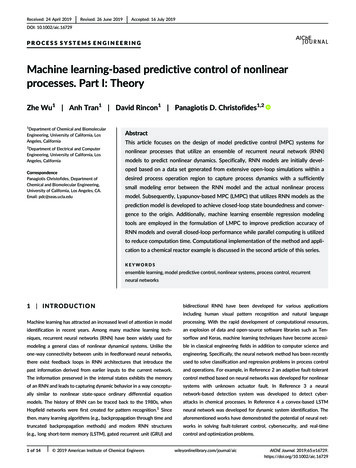
3 of 14WU ET AL.is, A\B: {x 2 Rn x 2 A, x 2B}. ; signifies the null set. The function f( )the control law φ(x). Φi(x) of Equation (3) represents the ith componentis of class C1 if it is continuously differentiable in its domain. A contin-of the saturated control law Φ(x) that accounts for the input constraintuous function α: [0,a) ! [0, ) is said to belong to class K if it is strictlyu 2 U. Based on Equation (2), we can first characterize a region whereincreasing and is zero only when evaluated at zero.the time-derivative of V is rendered negative under the controller Φ(x) 2noUasφu x 2 Rn j V ðxÞ Lf V Lg Vu kV ðxÞ, u ΦðxÞ 2 U [ f0g,2.2 Class of systemswhere k is a positive real number. Then the closed-loop stabilityThe class of continuous-time nonlinear systems considered isset of the Lyapunov function, which is inside φu: Ωρ : {x 2 φu region Ωρ for the nonlinear system of Equation (1) is defined as a leveldescribed by the following system of first-order nonlinear ordinaryV (x) ρ}, where ρ 0 and Ωρ φu. Also, the Lipschitz property of F(x,u,differential equations:w) combined with the bounds on u and w implies that there exist posi-x F ðx, u, wÞ f ðxÞ gðxÞu hðxÞw, xðt0 Þ x0ð1Þwhere x 2 Rn is the state vector, u 2 Rm is the manipulatedinput vector, and w 2 W is the disturbance vector with W {w 2 Rq w wm, wm 0}. The control action constraint is defined by u 2 U uimin ui uimax , i 1, , m Rm . f( ), g( ), and h( ) are sufficiently smooth vector and matrix functions of dimensions n 1, n m,and n q, respectively. Throughout the manuscript, the initial time t0tive constants M, Lx , Lw ,L0x , L0w such that the following inequalities holdfor all x, x'2 D, u 2 U, and w 2 W:j F ðx, u, wÞ j Mð4aÞj Fðx, u, wÞ F ðx0 , u, 0Þ j Lx j x x0 j Lw j w jð4bÞ V ðxÞ 0 V ðx0 Þ 0 L j x x0 j L0 j w jFðx,u,wÞ Fxð,u,0Þw x x xð4cÞis taken to be zero (t0 0), and it is assumed that f(0) 0, and thus,the origin is a steady state of the nominal (i.e., w(t) 0) system of Equation (1) (i.e., x*s , u*s ð0,0Þ, where x*s and u*s represent the3 R E C U RR E N T N E U R A L NE T W O R Ksteady-state state and input vectors, respectively).In this work, we develop an RNN model with the following form:2.3 Stabilization via control Lyapunov functionWe assume that there exists a stabilizing control law u Φ (x) 2 Ux F nn ðx , uÞ Ax ΘT yð5Þ25(e.g., the universal Sontag control law ) such that the origin of the nominal system of Equation (1) (i.e., w(t) 0) is rendered exponentially stablewhere x 2 Rn is the RNN state vector and u 2 Rm is the manipulatedin the sense that there exists a C1 Control Lyapunov function V (x) suchinput vector. y ½y1 , , yn , yn 1 , , ym n ½σ ðx 1 Þ, , σ ðx n Þ, u1 , , um that the following inequalities hold for all x in an open neighborhood2 Rn m is a vector of both the network state x and the input u, whereσ( ) is the nonlinear activation function (e.g., a sigmoid function σ(x) 1/D around the origin:(1 e-x)). A is a diagonal coefficient matrix, that is, A diag{ a1, ,c1 jxj2 V ðxÞ c2 jxj2 ,ð2aÞ an} 2 Rn n, and Θ [θ1, , θn] 2 R(m n) n with θi bi[wi1, ,wi(m n)], V ðxÞF ðx, ΦðxÞ, 0Þ c3 jxj2 , xð2bÞinput to the ith neuron where i 1, , n and j 1, , (m n). Addition- V ðxÞ x c4 j x jð2cÞi 1, , n. ai and bi are constants. wij is the weight connecting the jthally, ai is assumed to be positive such that each state x i is boundedinput bounded-state stable. Throughout the manuscript, we use x torepresent the state of actual nonlinear system of Equation (1) and usex for the state of the RNN model Equation (5).where c1, c2, c3, and c4 are positive constants. F(x,u,w) represents theUnlike the one-way connectivity between units in feedforwardnonlinear system of Equation (1). A candidate controller Φ(x) is givenneural networks (FNN), RNNs have signals traveling in both directionsin the following form:by introducing loops in the network. As shown in Figure 1, the statespffiffiffiffiffiffiffiffiffiffiffiffiffiffip p2 q4 q if q 6¼ 0φi ðxÞ qT q:0if q 08 minifφi ðxÞ uimin uiminΦi ðxÞ φi ðxÞ if ui φi ðxÞ uimax : maxuiifφi ðxÞ uimax8 information derived from earlier inputs are fed back into the network,ð3aÞwhich exhibits a dynamic behavior. Consider the problem of approximating a class of continuous-time nonlinear systems of Equation (1)by an RNN model of Equation 5. Based on the universal approxima-ð3bÞtion theorem for FNNs, it is shown in, for example, References 9 and20 that the RNN model with sufficient number of neurons is able toapproximate any dynamic nonlinear system on compact subsets ofwhere p denotes LfV (x) and q denotes LgiV (x), f [f1 fn]T, gi [gi1, ,the state-space for finite time. The following proposition demon-gin] , (i 1, 2, , m). φi(x) of Equation (3a) represents the ith component ofstrates the approximation property of the RNN model:T
4 of 14WU ET AL.for all x 2 Ωρ and u 2 U. It is noted that the modeling error ν(t) isbounded (i.e., ν(t) νm, νm 0) as x(t) and u(t) are bounded. Additionally, to avoid the weight drift problem (i.e., the weights go to infinityduring training), the weight vector θi is bounded by θi θm,where θm 0. Following the methods in References 10 and 28 theRNN learning algorithm is developed to demonstrate that the stateerror j e j j x x j is bounded in the presence of the modeling error ν.Specifically, the RNN model is identified in the form of Equation (5)and the nominal system of Equation (1) (i.e., w(t) 0) can be expressedF I G U R E 1 A recurrent neural network and its unfolded structure,where Θ is the weight matrix, x is the state vector, u is the inputvector, and o is the output vector (for the nonlinear system in theform of Equation (1), the output vector is equal to the state vector)[Color figure can be viewed at wileyonlinelibrary.com]Proposition 126Consider the nonlinear system of Equation (1) and theby the following equation:x i ai xi θ*Ti y νi , i 1, ,nThe optimal weight vector θ*i is defined as follows:θ*i arg min(NdXjθi j θm)jF i ðxk ,uk , 0Þ ai xk θTi yk jð8Þk 1RNN model of Equation (5) with the same initial conditionxð0Þ x ð0Þ x0 2 Ωρ . For any ε 0 and T 0, there exists an optimalð7Þwhere Nd is the number of data samples used for training. The stateweight matrix Θ* such that the state x of the RNN model of Equation (5)error is defined as e x x 2 Rn . Based on Equations (5) and (7), thewith Θ Θ * satisfies the following equation:time-derivative of state error is derived as follows:sup j xðtÞ x ðtÞ j ϵt2½0, T ð6Þe i x i x i ai ei ζTi y νi , i 1, , nð9ÞRemark 1 The RNN model of Equation (5) is developed as awhere ζi θi θ*i is the error between the current weight vector θi andcontinuous-time network as it is utilized to approximate the input–the unknown optimal weight vector θ*i . ν is the modeling error givenoutput behavior of the continuous-time nonlinear system of Equa-by ν F(x,u,0) Ax Θ*y. The weight vector θ is updated during thetion (1). As discussed in Reference 27 continuous-time RNNs havetraining process as follows:many advantages, for example, the well-defined derivative of theθ i ηi yei , i 1, , ninternal state with respect to time. However, it should be noted thatð10Þthe discrete-time RNNs can be equally well applied to model thewhere the learning rate η is a positive definite matrix. Based on thenonlinear system of Equation (1), where similar learning procedureslearning law of Equation (10), the following theorem is established toand stability analysis can also be derived. Additionally, in our work,demonstrate that the state error e remains bounded and is con-the RNN model of Equation (5) and the controller are both simulatedstrained by the modeling error ν.in a sample-and-hold fashion with a sufficiently small samplingperiod Δ.Theorem 1 Consider the RNN model of Equation (5) of which theweights are updated according to Equation (10). Then, the state errorei and the weight error ζi are bounded, and there exist λ 2 R and μ 03.1 RNN learning algorithmsuch that the following inequality holds:ðtIn this section, the RNN learning algorithm is developed to obtainthe optimal weight matrix Θ*, under which the error betweenthe actual state x(t) of the nominal system of Equation (1)(i.e., w(t) 0) and the modeled states x ðtÞ of the RNN of Equa-ðtjeðτÞj2 dτ λ μ jνðτÞj2 dτ0ð11Þ0 P Proof We first define a Lyapunov function V 12 ni 1 e2i ζTi ηi 1 ζi .:tion (5) is minimized. Although it is demonstrated in Proposition 1 thatBased on Equations (9) and (10) and ζi θ i , the time-derivative of V isRNNs can approximate a broad class of nonlinear systems to anyderived as follows:degree of accuracy, it is acknowledged that RNN modeling may notbe perfect in many cases due to insufficient number of nodes orn ::XV ei ei ηi 1 ζi ζ ilayers. Therefore, we assume that there exists a modeling errorν Fðx, u, 0Þ Fnn ðx , uÞ between the nominal system of Equation (1)and the RNN model of Equation (5) with Θ Θ*. As we focus on thesystem dynamics of Equation (1) in a compact set Ωρ, from which theorigin can be rendered exponentially stable using the controller u Φ(x) 2 U, the RNN model is developed to capture the system dynamics i 1n X ai e2i ei νi ð12Þi 1It is noted that in the absence of modeling error (i.e., νi 0), itholds that V 0. Following the proof in Reference 10 it is shown that
5 of 14WU ET AL.:the state error ei and its time-derivative ei are bounded for all times.adjust the weight such that the assumption that the weight vector θiAdditionally, as V is bounded from below and V is uniformly continu-is bounded by θi θm holds for all times. The switching ous implied by the fact that the second order derivative V is bounded,σ-modification approach was then improved to be continuous in theit follows that V ! 0 as t ! according to Barbalat's lemma.29 Thisimplies that ei ultimately converges to zero if there is no modelingconsidered compact set to overcome the problem of existence anduniqueness of solutions. The interested reader may refer to References 9 and 16 for further information.error term eiνi in Equation (12). However, in the presence of modeling error νi 6¼ 0, V 0 does not hold for all times. Therefore, based onEquation (12), the following equation is further derived:3.2 Development of RNN modelV nX i 1 αV ai 2 1 21 2 ai 2e jζ j jζ j ei ei νi2 i2 i 2 i2nX1 2ai 21 21 2ν νe ei νi jζ j 2 i2ai i2ai i2 ii 1 αV In this section, we discuss how to develop an RNN model fromscratch for a general class of nonlinear system of Equation (1) withinð13Þan operating region. Specifically, the development of a neural networkmodel includes the generation of dataset and the training process.nX1 2 1 2νjζ j 2 i2ai ii 13.2.1 Data generationwhere α : min{ai,1/(λm), i 1, , n} and λm represents the maximumeigenvalue of ηi 1 . As the weight vector is bounded by θi θm, it isderived that 12 jζ i j2 2θ2m , and it follows that V αV β, where P β ni 1 2θ2m ν2m 2ai . Therefore, V 0 holds for all V V0 β/α,Open-loop simulations are first conducted to generate the datasetthat captures the system dynamics for x 2 Ωρ and u 2 U as we focuson the system dynamics of Equation (1) in a compact set Ωρ with theconstrained input vector u 2 U. Given various x0 2 Ωρ, the open-loop it is readilywhich implies that V is bounded. From the definition of V,simulations of the nominal system of Equation 1 are repeated undershown that ei and ζ i are bounded as well. Moreover, based on the fact Pthat V ni 1 a2i e2i 2a1 i ν2i derived from Equation (13), we can alsovarious inputs u to obtain a large number of trajectories for finite time as follows:derive V(t)discretize the targeted region in state-space and the range of inputsðtð1 tei ðτÞ dτ νi ðτÞ2 dτ2ai 00i 1ððta min t1 V ð0Þ jeðτÞj2 dτ jνðτÞj2 dτ2a min 02 0V ðtÞ V ð0Þ to sweep over all the values that (x,u) can take. However, it is notedthat due to the limitation of computational resources, we may have tonXai 2with sufficiently small intervals in practice as shown in Figure 2. Sub-2sequently, time-series data from open-loop simulations can be sepað14Þrated into a large number of time-series samples with a shorter periodPnn, which represents the prediction period of RNNs. Lastly, thedataset is partitioned into training, validation, and testing datasets.Additionally, it should be noted that we simulate the continuouswhere amin is the minimum value of ai, i 1, ,n. Let λ 22 a min sup V ð0Þ V ðtÞ and μ 1 a min . The relationship between e andt 0system of Equation (1) under a sequence of inputs u 2 U in a sampleand-hold fashion (i.e., the inputs are fed into the system of Equation (1)as a piecewise constant function, u(t) u(tk), 8t 2 [tk, tk 1), where tk 1: μ shown in Equation 11 is derived as follows: tk Δ and Δ is the sampling period). Then, the nominal system ofðtjeðτÞj2 dτ 02 1V ð0Þ V ðtÞ 2a mina minðt λ μ jνðτÞj2 dτðt0Equation (1) is integrated via explicit Euler method with a sufficientlyjνðτÞj2 dτð15Þ0small integration time step hc Δ.Remark 3 In this study, we utilize the above data generation methodto obtain the dataset consisting of fixed-length, time-series state tra-Therefore, it is guaranteed that the state error e is bounded and isjectories within the closed-loop stability region Ωρ for the nonlinearproportional to the modeling error ν . Furthermore, it is noted that ifÐ there exists a positive real number C 0 such that 0 jνðtÞj2 dt C ,Ð then it follows that 0 jeðtÞj2 dt λ μC . As e(t) is uniformly contin-system of Equation (1). There also exist other data generationuous (i.e., ė is bounded), it implies that e(t) converges to zerolinearity behavior of system dynamics within the targeted region.asymptotically.However, regarding handling unstable steady-states, finite-lengthapproaches for data-driven modeling, for example, simulations underpseudo-random binary input signals (PRBS)30 that excite the non-open-loop simulations with various initial conditions x0 2 Ωρ outRemark 2 As the weights may drift to infinity in the presence ofperform the PRBS method in that the state trajectories can bemodeling error, a robust learning algorithm named switchingbounded in or stay close to Ωρ within a short period of time, whileσ-modification approach was proposed in References 9 and 16 tostates may diverge quickly under continuous PRBS inputs.
6 of 14WU ET AL.minimizing the modeling error ν is solved using adaptive moment estimation method (i.e., Adam in Keras) with the loss function calculatedby the mean squared error or the mean absolute percentage errorbetween predicted states x and actual states x from training data. Theoptimal number of layers and neurons are determined through a gridsearch. Additionally, to avoid over-fitting of the RNN model, the training process is terminated once the modeling error falls below thedesired threshold and the early-stopping condition is satisfied (i.e., theerror on the validation set stops decreasing).Remark 4 In some cases training datasets may consist of noisy dataor corrupt data, which could affect the training performance of RNNsin the following manners. On the one hand, noise makes it more challenging for RNNs to fit data points precisely. On the other hand, it isshown in Reference 20 that the addition of noise can also improvegeneralization performance and robustness of RNNs, and sometimeseven lead to faster learning. Therefore, the neural network trainingwith noise remains an important issue that needs further investigation. However, in our work, it should be noted that the open-loop simulations are performed for the nominal system of Equation (1) (i.e., w(t) 0) only. Based on the noise-free dataset, the RNN models areF I G U R E 2 The schematic of discretization of the operating regionΩρ and the generation of training data for RNNs with a predictionperiod Pnn for all initial conditions x0 2 Ω ρ, where hc is the timeinterval between RNN internal states, Ωρ is the closed-loop stabilityregion for the actual nonlinear system of Equation (1) and Ωρ is theclosed-loop stability region characterized for the obtained RNN model[Color figure can be viewed at wileyonlinelibrary.com]trained to approximate the dynamics of the nominal system of Equation (1) within the closed-loop stability region Ωρ . Additionally,although the RNN model is derived for the nominal system of Equation (1), it will be shown in Section “Sample-and-hold Implementationof Lyapunov-based Controller” that the obtained RNN models can beapplied with model predictive control to stabilize the nonlinear systemof Equation (1) in the presence of small bounded disturbances(i.e., w wm).3.2.2 Training processRemark 5 In our study, the operating region considered is chosen asNext, the RNN model is developed using a state-of-the-art applicationthe closed-loop stability region Ωρ that is characterized for the first-program interface (API), that is, Keras.31 The prediction period ofprinciples model of Equation (1), in which there exist control actionsRNN, Pnn, is chosen to be an integer multiple of the sampling period Δu 2 U that render the steady state of Equation (1) exponentially stablesuch that the RNN model Fnn ðx ,uÞ can be utilized to predictfor all x0 2 Ωρ. However, in the case that the closed-loop stabilityfuture states for at least one sampling period by taking state measure-region Ωρ for the first-principles model of Equation (1) is unknown,ment x(tk) and manipulated inputs u(tk) at time t tk. As shown inthe operating region Ωρ for collecting data can be initially character-Figure 2, within the RNN prediction period Pnn, the time intervalized as a sufficiently large set around the steady state containing allbetween two consecutive internal states xt-1 and xt for the unfoldedthe states that the system might move to. This operating region mayRNN shown in Figure 1 is chosen to be the integration time step hcbe larger than the actual closed-loop stability region Ωρ, and therefore,used in open-loop simulations. Therefore, all the states between t 0it is likely that no control actions u 2 U exist to drive the state towardand t Pnn with a step size of hc are treated as the internal states andthe origin for some initial conditions x0 in this operating region. How-can be predicted by the RNN model. Based on the dataset generatedever, this problem can be overcome through the recharacterization offrom open-loop simulations, the RNN model of Equation (5) is trainedthe closed-loop stability region Ωρ after the RNN is obtained. Specifi-to calculate the optimal weight Θ* of Equation (8) by minimizing thecally, based on the dataset generated in this operating region, themodeling error between F(x,u,0) and F nn ðx , uÞ. Furthermore, to guaran-RNN model is derived following the training approach in this section,tee that the RNN model of Equation (5) achieves good performance inand subsequently, the actual operating region (i.e., the closed-loopa neighborhood around the origin and has the same equilibrium pointstability region Ωρ for the RNN model of Equation (5)) will be charac-as t
model predictive control (MPC). As an advanced control methodology, MPC has been applied in real-time operation of industrial chemical plants to optimize process performance accounting for process stabil-ity, control actuator, and safety/state constraints.5,6 One key require-ment of MPC is the availability of an accurate process model to .